Week 7 - Simulation of a 1D Super-sonic nozzle flow simulation using Macormack Method
*AIM:-
Simulation of a quasi 1D Super-sonic nozzle flow simulation using Macormack Method
*Objective:-
We are going to simulate the isentropic flow through a quasi 1D subsonic-supersonic nozzle. We will derive both the conservation and non-conservation forms of the governing equations and sovle them using the MacCormack's technique. We need to determine the steady-state temperature distribution for the flow-field variables and investigate the difference between the two forms of governing equations by comparing their solutions.
*Introdution:-
-Nozzle is a one type of device which is use for control the direction or charasteristics of a fluid flow(mass, pressure, speed, shape etc). This change are posible due to vary of cross section area of the nozzle.
-In this case we use convergent-divergent nozzle. The flow at the inlet at the nozzle come from reservoir where pressure and temperature are constant.The cross-section are of reservoir is so large then the velocity at the inlet is almost zero.
-The flow expand isentropically to supersonic speeds at nozzle exist.
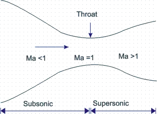
*The speed is devided in to the three parts:-
i) Subsonic speed:-
-If speed of flows are lessthan the speed of sound is called subsonic speed.
-For that mack numberis lessthan 1.(M<1)
ii) Sonic speed:-
-If speed of flows are equal to the speed of sound is called sonic speed.
-For that mack number is equal to 1. (M=1)
iii) Supersonic speed:-
-If speed of flows are morethan the speed of sound is called supersonic speed.
-For that mack numberis morethan 1.(M>1)
Note:-In this case the flows are subsonic in the convergent section , subsonic at throat and supersonic in divergent section.
*What do you means of Quasi 1D problem:-
-Actually nozzle problem is a 3-D problem. Beacusefluids are go every direction in the nozzle. That thing we understand by the figure.
-But its complicated problem, So for simplification we assume its 1-D only. It means here we assume fluid flow is does not vary in y-direction. Its vary in only x-direction. So this is called Quasi 1-D problem.
*Conservative form and non-conservative form:-
-If we solve governing equation numerically then we required equation in form of intergal.Because we write the program in the computer and its understand the intergral form, not a PDE form.
-When you solve the equation numerically (means discretize and solving using computer) then error propagate. Due to that two form generate. 1) Coservative form, 2) Non conservative form.
-This forms are analytically same, but numerically different.
1) Conservative form:-
-The equation obtain from finite control volume fixed in space is called conservative form.
-In this case control volume is stationary.
2) Non censervative form:-
-The equations obtain from finite control volume moving with fluid is called nonconservative form.
*Maccormack's techiques:-
-This method is improved to solve quasi 1D supersonic nozzle flow rather than use of differencing scheme.
-It is a explicit finite difference technique which second order accurate in both time and space.
-This technique is devided in to three parts, and is called step.
1) Predicted step
2) Corrected step
3) Final step
*For nonconservative method:-
1) Predicted step:-
-In the predicted step the spatial term on the right hand side of the equations are replaced by forward difference scheme.
-The right hand side of the equation is known as all the value of variables for time step t.
-Next the value of variable on the LHS is calculated by employing the time marching solution.
*For continuity equation:-
`(∂ρ)/(∂t)=-ρ (∂v)/(∂x)-ρv ∂/(∂x) (lnA)-v (∂ρ)/(∂x)`
`(ρ_i^(n+1)-ρ_i^n)/(∆t)=-ρ_i^n [(v_(i+1)^n-v_i^n)/(∆x)]-ρ_i^n v_i^n [(ln(A_(i+1) )-ln(A_i ))/(∆x)]-v_i^n [(ρ_(i+1)^n-ρ_i^n)/(∆x)]`
We find the `((∂ρ)/(∂t))_i``((∂v)/(∂t))_i` and `((∂T)/(∂t))_i`for predictor.
`(ρ_i)^(update)=(ρ_i)^(i.c.)+((∂ρ)/(∂t))_i×dt`
2) Corrected step:-
`((∂ρ)/(∂t))_i=-ρ_i^u [(v_i^u-v_(i-1)^u)/(∆x)]-ρ_i^u v_i^u [(ln(A_(i+1) )-ln(A_i ))/(∆x)]-v_i^u [(ρ_(i+1)^u-ρ_i^u)/(∆x)]`
-It is same for `((∂v)/(∂t))_i` and `((∂T)/(∂t))_i`for correced step.
3) Final step:-
`((∂ρ)/(∂t))_(avg)=0.5×[((∂ρ)/(∂t))_(predicted)+((∂ρ)/(∂t))_(corectrd)]`
-It is same for `((∂v)/(∂t))_(avg)` and `((∂T)/(∂t))_(avg)`for correced step.
-After complete of this three stpes we solve density, velocity and temperature for next timestep.
`(ρ_i)^(sec)=ρ_i^(first)+((∂ρ)/(∂t))_(avg)×dt`
-This steps similary apply for the momentum equation and energy equation.
*momentum equation:-
`(∂v)/(∂t)=-v (∂v)/(∂x)-1/γ((∂T)/(∂x)+T/ρ (∂p)/(∂x))`
*Energy equation:-
`(∂T)/(∂t)=-v (∂T)/(∂x)-(γ-1)T((∂v)/(∂x)+v (∂(lnA))/(∂x))`
*For conservative method:-
1) Continuity equation:-
`(∂(ρA))/(∂t)+(∂(ρAv))/(∂x)=0∂t`
2) Momentum equation:-
`(∂(ρAv))/(∂t)+∂/(∂x)[ρAv^2+1/γ ρA]=1/γ ρ (∂A)/(∂x) ∂t`
3) Energy equation:-
`∂/(∂t) [ρ(T/(γ-1)+γ/(2v^2 )A]+∂/(∂x)[ρ(T/(γ-1)+γ/(2v^2 )vA+ρAv]=0∂t`
*Boundary condition:-
-Boundary condition and initial condition are most important part in any simulation. So we provide the boundary condition.
*Inlet boundary condition:-
`v_1=2×v_2-v_3`
*Outlet boundary condition:-
`v_n=2×v_(n-1)-v_(n-2)`
-Its similary for temperature and density.
`T_n=2×T_(n-1)-T_(n-2)`
`ρ_n=2×ρ_(n-1)-ρ_(n-2)`
*Matlab script file:-
1) Main file:-
clear all
close all
clc

%initial condition
%number of nodes in x-direction
n=31;
x=linspace(0,3,n);
%distance between two gradual nodes
dx=x(2)-x(1);
CFL=0.5;
tol=1e-6;

a=1+2.2*(x-1.5).^2;

n_throat=find((a-1)<1e-3);
gamma=1.4;

%non conservative solver
tic;
[rho_ncon,T_ncon,v_ncon,p_ncon,M_ncon,massflow_ncon,rho_throat_ncon,p_throat_ncon,T_throat_ncon,M_throat_ncon,k_ncon]=non_conservative_solver(x,dx,n,a,CFL,tol,n_throat,gamma)
time_nc=toc;

%conservative solver
tic;
[rho_con,T_con,v_con,p_con,M_con,massflow_con,rho_throat_con,p_throat_con,T_throat_con,M_throat_con,k_con]=conservative_solver(x,dx,n,a,CFL,tol,n_throat,gamma)
time_c=toc;

%ploting results
%transient throat profile
figure(3)
subplot(4,1,1)
plot(rho_throat_ncon,'m');
hold on;
plot(rho_throat_con,'k');
legend('Non conservative form','Conservative form');
ylabel('rho');
title('Timewise variation of fluid properties at troat of nozzle');
title('variation of density ratio');
axis([0 k_ncon 0.5 1]);
grid minor;

subplot(4,1,2)
plot(T_throat_ncon,'r');
hold on
plot(T_throat_con,'y');
legend('Non conservative form','Conservative form');
ylabel('T');
title('variation of temperature ratio');
axis([0 k_ncon 0.6 1.2]);
grid minor;

subplot(4,1,3)
plot(p_throat_ncon,'g');
hold on
plot(p_throat_con,'k');
legend('Non conservative form','Conservative form');
ylabel('p');
title('variation of pressure ratio');
axis([0 k_ncon 0.4 1]);
grid minor;

subplot(4,1,4)
plot(M_throat_ncon,'r');
hold on
plot(T_throat_con,'b');
legend('Non conservative form','Conservative form');
ylabel('M');
title('variation of Mach number');
axis([0 k_ncon 0.8 1.8]);
grid minor;
xlabel('number of interations');

%steady state profile
figure(4)
subplot(4,1,1)
plot(x,rho_ncon,'m',x,rho_con,'k*');
legend('non conservative form','conservative form');
title('variation of fluid properties across the nozzle');
title('variation of density ratio');
ylabel('rho');
grid minor;

subplot(4,1,2)
plot(x,T_ncon,'m',x,T_con,'k*');
legend('non conservative form','conservative form');
title('variation of temperature ratio');
ylabel('T');
grid minor;

subplot(4,1,3)
plot(x,p_ncon,'m',x,p_con,'k*');
legend('non conservative form','conservative form');
title('variation of pressure ratio');
ylabel('p');
grid minor;

subplot(4,1,4)
plot(x,M_ncon,'m',x,M_con,'k*');
legend('non conservative form','conservative form','location','southeast');
title('variation of Mach number');
ylabel('M');
grid minor;
xlabel('x');

%comarision of steady massflow rate
figure(5)
plot(x,massflow_ncon);
hold on
plot(x,massflow_con);
hold on
ana_sol=0.579*ones(1,n);
plot(x,ana_sol,'r');
title('comaprision of steady massflow profile');
legend('non conservativeform','conservative form','analytical solution');
grid minor;
axis([0 3 0.575 0.6])
2) User define function for nonconservative form:-
function [rho,T,v,p,M,massflow,rho_throat,p_throat,T_throat,M_throat,k]=non_conservative_solver(x,dx,n,a,CFL,tol,n_throat,gamma)

%initial profiles and value
%density
rho=1-0.3146*x;
%temperature
T=1-0.2314*x;
%velocity
v=(0.1+1.09*x).*T.^0.5;
%error term
error=1e9;
%starting time step
k=0;

while (error>tol)
      k=k+1;
      %storing old value
      rho_old=rho;
      T_old=T;
      v_old=v;
      sonic_speed=sqrt(T_old);
      massflow_old=rho_old.*v_old.*a;
      %CFL condition
      timestep=CFL*dx./(sonic_speed+v_old);
      dt=min(timestep);

      %predator step
      for i=2:n-1
          %creating forward difference term
          drhodx=(rho(i+1)-rho(i))/dx;
          dvdx=(v(i+1)-v(i))/dx;
          dTdx=(T(i+1)-T(i))/dx;
          dlogadx=(log(a(i+1))-log(a(i)))/dx;

          %continuity equation
          drhodt_p(i)=-(rho(i)*dvdx+rho(i)*v(i)*dlogadx+v(i)*drhodx);

          %momentum equation
          dvdt_p(i)=-(v(i)*dvdx+((1/gamma)*(dTdx+(T(i)/rho(i))*drhodx)));

          %energy equation
          dTdt_p(i)=-(v(i)*dTdx+(gamma-1)*T(i)*(dvdx+v(i)*dlogadx));

          %solution update
          rho(i)=rho(i)+drhodt_p(i)*dt;
          v(i)=v(i)+dvdt_p(i)*dt;
          T(i)=T(i)+dTdt_p(i)*dt;
      end

      %corrector step
      for i=2:n-1
            %creating backword difference term
            drhodx=(rho(i)-rho(i-1))/dx;
            dvdx=(v(i)-v(i-1))/dx;
            dTdx=(T(i)-T(i-1))/dx;
            dlogadx=(log(a(i))-log(a(i-1)))/dx;

            %continuity equation
            drhodt_c(i)=-(rho(i)*dvdx+rho(i)*v(i)*dlogadx+v(i)*drhodx);

            %momentum equation
            dvdt_c(i)=-(v(i)*dvdx+((1/gamma)*(dTdx+(T(i)/rho(i))*drhodx)));

            %energy equaction
            dTdt_c(i)=-(v(i)*dTdx+(gamma-1)*T(i)*(dvdx+v(i)*dlogadx));
      end

      %complete time derivative
      drhodt=0.5*(drhodt_p+drhodt_c);
      dTdt=0.5*(dTdt_p+dTdt_c);
      dvdt=0.5*(dvdt_p+dvdt_c);

      %next timestep value
      for i=2:n-1
            rho(i)=rho_old(i)+drhodt(i)*dt;
            v(i)=v_old(i)+dvdt(i)*dt;
            T(i)=T_old(i)+dTdt(i)*dt;
      end

      %applying boundary condition
      %inlet
      v(1)=2*v(2)-v(3);
      rho(1)=1;
      T(1)=1;

      %outlet
      v(n)=2*v(n-1)-v(n-2);
      rho(n)=2*rho(n-1)-rho(n-2);
      T(n)=2*T(n-1)-T(n-2);

      %calculating variables
      M=v./(sqrt(T));
      p=rho.*T;
      massflow=rho.*v.*a;

      %transient throat value
      rho_throat(k)=rho(n_throat);
      p_throat(k)=p(n_throat);
      M_throat(k)=M(n_throat);
      T_throat(k)=T(n_throat);

      %checking for convergence
      error=max(abs(massflow-massflow_old));

    %nontransient mass flow rate at various time step
    figure(1)
    hold on
    if k==1
      plot(x,massflow,'color','k');
    else if k==50
      plot(x,massflow,'color','g');
    else if k==100
      plot(x,massflow,'color','r');
    else if k==200
      plot(x,massflow,'color','b');
    else if k==400
      plot(x,massflow,'color','y');
    else if k==900
      plot(x,massflow,'color','m');
      plot(x(end),massflow(end),'k*');
    end
    end
    end
    end
    end
    end
    end

    title('non conservative analysis');
    xlabel('x/L');
    ylabel('rho*a*v');
    legend('0','50','100','200','400','900');
    axis([0 3 0 2]);
    grid minor;
end
3) User define function for conservative form:-
function [rho,T,v,p,M,massflow,rho_throat,p_throat,T_throat,M_throat,k]=non_conservative_solver(x,dx,n,a,CFL,tol,n_throat,gamma)

%initial profiles and value
%density
rho=1-0.3146*x;
%temperature
T=1-0.2314*x;
%velocity
v=(0.1+1.09*x).*T.^0.5;
%error term
error=1e9;
%starting time step
k=0;

while (error>tol)
      k=k+1;
      %storing old value
      rho_old=rho;
      T_old=T;
      v_old=v;
      sonic_speed=sqrt(T_old);
      massflow_old=rho_old.*v_old.*a;
      %CFL condition
      timestep=CFL*dx./(sonic_speed+v_old);
      dt=min(timestep);

      %predator step
      for i=2:n-1
          %creating forward difference term
          drhodx=(rho(i+1)-rho(i))/dx;
          dvdx=(v(i+1)-v(i))/dx;
          dTdx=(T(i+1)-T(i))/dx;
          dlogadx=(log(a(i+1))-log(a(i)))/dx;

          %continuity equation
          drhodt_p(i)=-(rho(i)*dvdx+rho(i)*v(i)*dlogadx+v(i)*drhodx);

          %momentum equation
          dvdt_p(i)=-(v(i)*dvdx+((1/gamma)*(dTdx+(T(i)/rho(i))*drhodx)));

          %energy equation
          dTdt_p(i)=-(v(i)*dTdx+(gamma-1)*T(i)*(dvdx+v(i)*dlogadx));

          %solution update
          rho(i)=rho(i)+drhodt_p(i)*dt;
          v(i)=v(i)+dvdt_p(i)*dt;
          T(i)=T(i)+dTdt_p(i)*dt;
      end

      %corrector step
      for i=2:n-1
            %creating backword difference term
            drhodx=(rho(i)-rho(i-1))/dx;
            dvdx=(v(i)-v(i-1))/dx;
            dTdx=(T(i)-T(i-1))/dx;
            dlogadx=(log(a(i))-log(a(i-1)))/dx;

            %continuity equation
            drhodt_c(i)=-(rho(i)*dvdx+rho(i)*v(i)*dlogadx+v(i)*drhodx);

            %momentum equation
            dvdt_c(i)=-(v(i)*dvdx+((1/gamma)*(dTdx+(T(i)/rho(i))*drhodx)));

            %energy equaction
            dTdt_c(i)=-(v(i)*dTdx+(gamma-1)*T(i)*(dvdx+v(i)*dlogadx));
      end

      %complete time derivative
      drhodt=0.5*(drhodt_p+drhodt_c);
      dTdt=0.5*(dTdt_p+dTdt_c);
      dvdt=0.5*(dvdt_p+dvdt_c);

      %next timestep value
      for i=2:n-1
            rho(i)=rho_old(i)+drhodt(i)*dt;
            v(i)=v_old(i)+dvdt(i)*dt;
            T(i)=T_old(i)+dTdt(i)*dt;
      end

      %applying boundary condition
      %inlet
      v(1)=2*v(2)-v(3);
      rho(1)=1;
      T(1)=1;

      %outlet
      v(n)=2*v(n-1)-v(n-2);
      rho(n)=2*rho(n-1)-rho(n-2);
      T(n)=2*T(n-1)-T(n-2);

      %calculating variables
      M=v./(sqrt(T));
      p=rho.*T;
      massflow=rho.*v.*a;

      %transient throat value
      rho_throat(k)=rho(n_throat);
      p_throat(k)=p(n_throat);
      M_throat(k)=M(n_throat);
      T_throat(k)=T(n_throat);

      %checking for convergence
      error=max(abs(massflow-massflow_old));

    %nontransient mass flow rate at various time step
    figure(1)
    hold on
    if k==1
      plot(x,massflow,'color','k');
    else if k==50
      plot(x,massflow,'color','g');
    else if k==100
      plot(x,massflow,'color','r');
    else if k==200
      plot(x,massflow,'color','b');
    else if k==400
      plot(x,massflow,'color','y');
    else if k==900
      plot(x,massflow,'color','m');
      plot(x(end),massflow(end),'k*');
    end
    end
    end
    end
    end
    end
    end

    title('non conservative analysis');
    xlabel('x/L');
    ylabel('rho*a*v');
    legend('0','50','100','200','400','900');
    axis([0 3 0 2]);
    grid minor;
end
*Results and discussion:-
-First of all we compare the results obtained from the non conservation and conservation analysis.
1) Evaluation of dimensionless massflow profile over time:-
i) For non conservative analysis:-
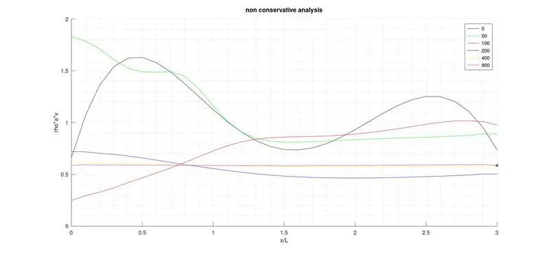
-This is actually error parameter that was used to check for convergence for time loop.
-The non dimensional mass flow is plotted as a function of non dimensional distance through the nozzle at different time step in the graph during the time marching procedure.
-Here the first curve is the variation of profile at the initial conditions.
-Finally we can seen that at 900 interations achieve the almost constant mass flow profile.
ii) For conservative analysis:-
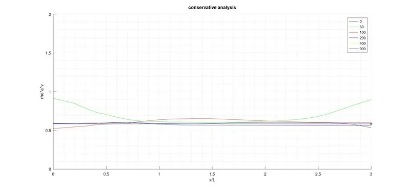
-Non conservative form and conservative form has diifferent initial condition, due to that we get a different mass flow rate curve compare to non conservative analysis.
-Values of every curves are near to each other and its closer to analytical value.(0.579) It means more mass is preserved in the conservative form than the non conservative form.
2) Variation of transient fluid properties at CD throat:-
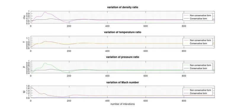
-Here the stability of the conservative and non conservative form solver has been demostreted.
-Initially value of the all parameters very high and there are oscilations, this occurs due to the various effect causes by expansion and compression . During the first few interations dumped out, solution approach near to stabilized constant condition.
3) Comparision of both form's mass flow rate and analytical result:-
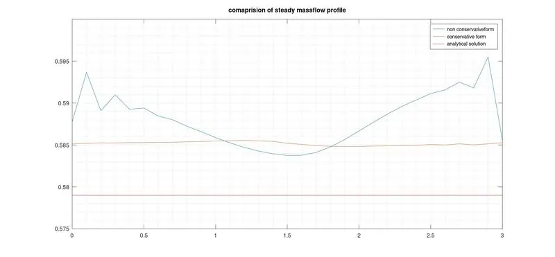
-Here study mass flow profiles are compared. This figure illustrates a general advantage of conservation form of equation.
-This form allways does a better job of preserving mass throughout the flow field. The conservative form gives mass flow rate variation that is close to constant value and more accurate result at steady state.
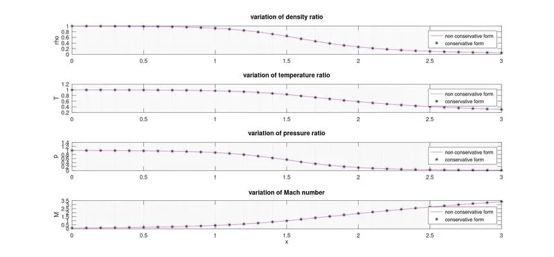
4) Variation of flow properties after approaching steady state condition:-
*Conclusion:-
-The non conservative form is faster than the conservative form and accuracy of the solution increase as we increase the number of grid points.
-The solution converge after the 900 time steps.
-For the same number of grid points non conservative form yields better result compare to the conservative form.
-Conservative dorm and non conservative form return the almost identical profile.