Week 7 - Simulation of a 1D Super-sonic nozzle flow simulation using Macormack Method
1. Aim:-
1. To simulate the isentropic flow through a quasi 1D subsonic-supersonic nozzle.
2. Derive conservative and non-conservative form of governing equations and solve them using MacCormack's method.
3. Determine the steady-state temperature distribution for the flow-field variables and investigate the difference between the two forms of governing equations by comparing their solutions.
2. Objective:-
1. Steady-state distribution of primitive variables inside the nozzle.
2. Time-wise variation of the primitive variables.
3. Variation of Mass flow rate distribution inside the nozzle at different time steps during the time-marching process.
4. Comparison of Normalized mass flow rate distributions of both forms.
3. Isentropic flow:-
In fluid dynamics, an isentropic flow is a fluid flow that is both adiabatic and reversible. That is, no heat is added to the flow, and no energy transformations occur due to friction or dissipative effects.
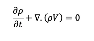
Conservative form of governing equation:-
Non-Conservative form of governing equation:-
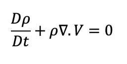
Theoretically and mathematically, there is no difference between conservative and non-conservative form but numerically there is huge difference between these forms.
The first difference that can be noticed between both forms is in the time derivative term. The local derivative in the conservation form is replaced with a substantial derivative in the non-conservation. In the conservation form, we make the derivation under the assumption that the control volume is fixed. So the variation of density with time is given by the local derivative. But in the non-conservation form, the control volume is assumed to be moving. In this case, the time rate of change of density will be the sum of local derivative (variation due to unsteady nature) and the convective derivative (variation due to moving control volume).
The second difference that can be noticed is the position of the ∇ operator. An interesting point to note in the continuity equation in conservation form is that the quantity that the divergence operator is acting on (i.e., ) is nothing but the mass flux (the rate of mass flow per unit area or the momentum per unit volume) which makes sense only when the control-volume is not moving. This feature continues to occur in the momentum and energy equations as well where the divergence operator acts on momentum flux and energy flux. The differences mentioned above help us distinguish conservation form against the non-conservation form of equations.
Introduction to the Physical problem: Subsonic-Supersonic isentropic flow
We consider the steady, isentropic flow through a convergent-divergent nozzle. The flow at the inlet to the nozzle comes from a reservoir where the temperature are denoted by To and po ,respectively. The cross sectional area of the reservoir is large (theoretically, A is ∞), and hence the velocity is very small. The flow expands isentropically to supersonic speeds at the nozzle exit, where the exit pressure, temperature, velocity, and Mach number are denoted by pe, Te, Ve, and Me, respectively. The flow is locally subsonic in the convergent section of the nozzle, sonic at the throat (minimum area), and supersonic at the divergent section. The sonic flow (M=1) at the throat means that the local velocity at this location is equal to the local speed of sound. The velocity, pressure, temperature and area at the throat are denoted by V*, p*, T* and A*, respectively. We make the assumption that the flow properties vary only with x, this is tantamount to make the assumption that the flow properties across any given cross-section. Such flow is defined as quasi-one-dimensional flow.
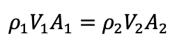
The governing continuity, momentum, and energy equations for this quasi-one dimensional, steady, isentropic flow can be expressed, respectively, as
Continuity:-
Momentum:-

Energy:-
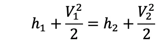
where subscripts 1 and 2 denote different locations along the nozzle.
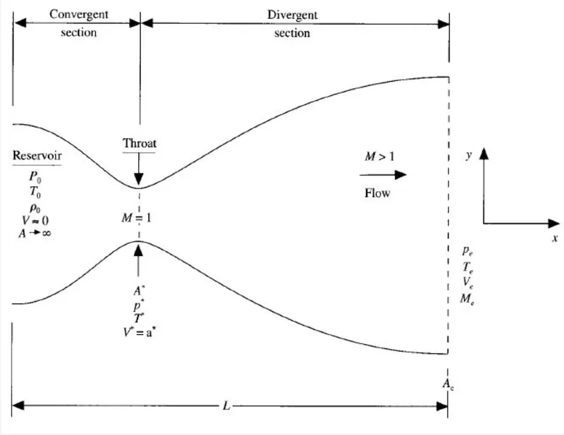
Above figure shows the 1D quasi nozzle flow.
The convergent-divergent nozzle is specified by a symmetrical area function as:

4. MacCormack's method
MacCormack's method is an explicit finite-difference technique which is second-order accurate in both space and time. Consider the two dimensional grid as shown in figure below
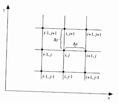
We assume that the flow field at each grid point in above figure is known at time t, and we proceed to calculate the flow-field variables at the same grid points at time t+Δt. First consider the density at grid point(i.j) at time t+Δt. In MacCormack's method, this is obtained from
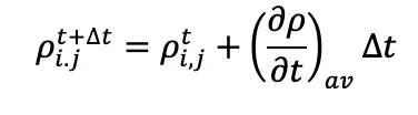
where (∂ρ/∂t)avg is a representative mean value of (∂ρ/∂t) between times t and t+Δt.
Similar relations are written for the other flow-field variables. i.e.,
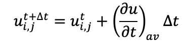
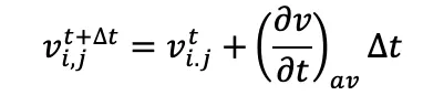
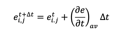
By using above method, we get the idea of using MacCormack's method. In MacCormack's method two steps are involved. One is Predictor method and another one is Corrector method.
5. a.) Non-conservative form:-
The non-conservative form of the governing equations which represent continuity, momentum and energy in terms of non-dimensional variables are:-
Continuity:
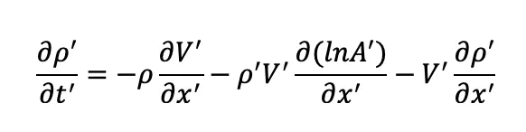
Momentum:
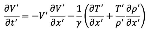
Energy:
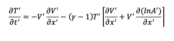
Non-Dimensional variables are:
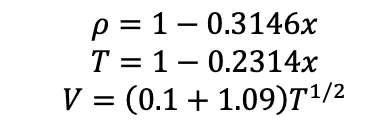
The initial conditions at t = 0 according to Anderson's book:
b.) Conservative form
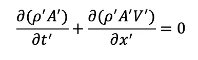
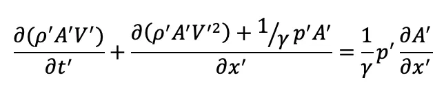
The conservative form of the governing equations which represent continuity, momentum and energy in terms of non-dimensional variables are:-
Continuity:
Momentum:
Energy:

Let us define the elements of the solutions vector U, the flux vector F, and the source term J as follows.
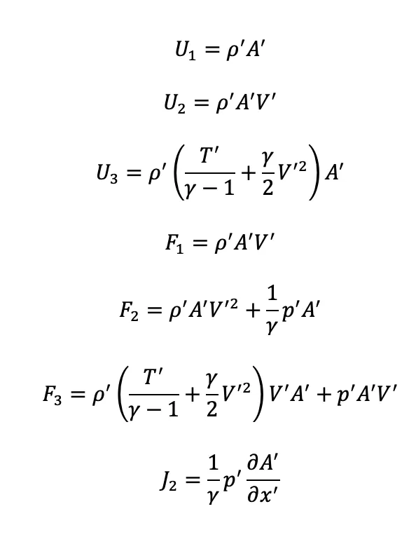
Therefore, governing equation can be written as:-
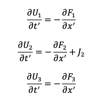
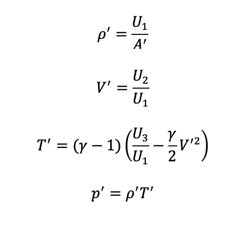
Our numerical numbers will give us numbers directly for U1, U2, and U3 in steps of time, this is why U is called the solutions vector. To obtain the primitive variables (𝜌, V, T, p, etc), we must decode the elements as follows,
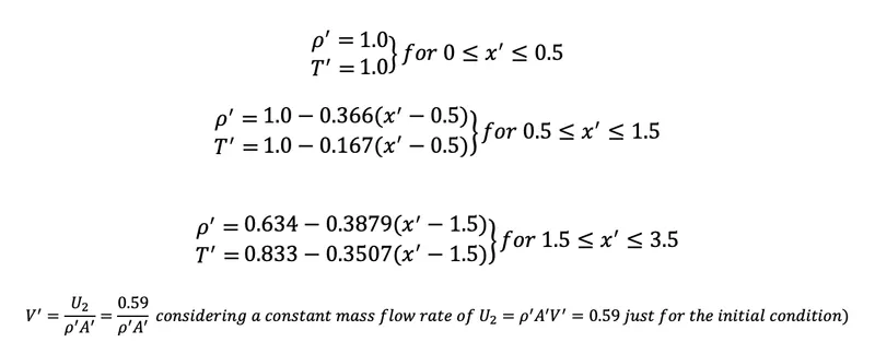
The Initial conditions for the conservative form of the equations are based on Anderson's book:
Matlab code: -
Main programme
clear all
close all
clc

%inputs
L = 3;
n = 31;
x = linspace(0,L,n);
dx = x(2) - x(1);
gamma = 1.4;
C = 0.5;
nt = 1400;

%nozzle area profile

a = 1 + 2.2*((x - 1.5).^2);
throat = find(a == 1);

% computing flow variables using non_conservative_method
[rho1, v1, t1, p1, M1, m1, rho_t_nc, v_t_nc, p_t_nc, t_t_nc, M_t_nc] = non_conservative_nozzle_1D_quassi(x, dx, C, nt, gamma, n, a, throat);

% computing solution vector using conservative_method
[rho, v, t, p, M, m, rho_t, v_t, p_t, t_t, M_t] = conservative_nozzle_1D_quassi(x, dx, C, nt, gamma, n, a, throat);


% plotting the results
figure(1)
subplot(4,1,1)
plot(x,M1,'LineWidth',2)
grid minor;
ax = gca;
ax.FontSize = 14;
ylim([0 4.5]);
yticks(0:1.5:4.5);
ylabel('Mach Number','FontSize',16,'FontWeight','bold')
title('Flow parameters using the non-conservative form of governing equation','FontWeight','bold','FontSize',28);
subplot(4,1,2)
plot(x,p1,'LineWidth',2)
grid minor;
ax = gca;
ax.FontSize = 14;
yticks(0:0.2:1);
ylabel('Pressure ratio','FontSize',16,'FontWeight','bold')
subplot(4,1,3)
plot(x,rho1,'LineWidth',2)
grid minor;
ax = gca;
ax.FontSize = 14;
ylim([0 1]);
yticks(0:0.2:1)
ylabel('Density ratio','FontSize',16,'FontWeight','bold')
subplot(4,1,4)
plot(x,t1,'LineWidth',2)
grid minor;
ax = gca;
ax.FontSize = 14;
ylim([0 1]);
yticks(0:0.2:1);
ylabel('Temperature ratio','FontSize',16,'FontWeight','bold')
xlabel('X/L','FontSize',20,'FontWeight','bold')

figure(2)
subplot(4,1,1)
plot(x,M,'LineWidth',2)
grid minor;
ax = gca;
ax.FontSize = 14;
ylim([0 4.5]);
yticks(0:1.5:4.5);
ylabel('Mach Number','FontSize',16,'FontWeight','bold')
title('Flow parameters using the conservative form of governing equation','FontWeight','bold','FontSize',28);
subplot(4,1,2)
plot(x,p,'LineWidth',2)
grid minor;
ax = gca;
ax.FontSize = 14;
yticks(0:0.2:1);
ylabel('Pressure ratio','FontSize',16,'FontWeight','bold')
subplot(4,1,3)
plot(x,rho,'LineWidth',2)
grid minor;
ax = gca;
ax.FontSize = 14;
yticks(0:0.2:1);
ylabel('Density ratio','FontSize',16,'FontWeight','bold')
subplot(4,1,4)
plot(x,t,'LineWidth',2)
grid minor;
ax = gca;
ax.FontSize = 14;
ylim([0 1]);
yticks(0:0.2:1)
ylabel('Temperature ratio','FontSize',16,'FontWeight','bold')
xlabel('X/L','FontSize',20,'FontWeight','bold')

figure(3)
subplot(4,1,1)
plot(1:nt,rho_t_nc,'LineWidth',2)
hold on
plot(1:nt,rho_t,'LineWidth',2)
grid minor;
ax = gca;
ax.FontSize = 14;
ylim([0 1]);
yticks(0:0.2:1);
ylabel('rho/rho_0','FontSize',16,'FontWeight','bold')
title('Flow parameter variation at the nozzle throat','FontWeight','bold','FontSize',28)
lgd = legend('Non-Conservative','Conservative');
lgd.FontSize = 16;
subplot(4,1,2)
plot(1:nt,t_t_nc,'LineWidth',2)
hold on
plot(1:nt,t_t,'LineWidth',2)
grid minor;
ax = gca;
ax.FontSize = 14;
yticks(0:0.2:1);
ylabel('t/t_0','FontSize',16,'FontWeight','bold')
lgd = legend('Non-Conservative','Conservative');
lgd.FontSize = 16;
subplot(4,1,3)
plot(1:nt,p_t_nc,'LineWidth',2)
hold on
plot(1:nt,p_t,'LineWidth',2)
grid minor;
ax = gca;
ax.FontSize = 14;
yticks([0:0.2:1]);
ylabel('p/p_0','FontSize',16,'FontWeight','bold')
lgd = legend('Non-Conservative','Conservative');
lgd.FontSize = 16;
subplot(4,1,4)
plot(1:nt,M_t_nc,'LineWidth',2)
hold on
plot(1:nt,M_t,'LineWidth',2)
grid minor;
ax = gca;
ax.FontSize = 14;
yticks([0:0.2:1]);
ylabel('mach number','FontSize',16,'FontWeight','bold')
xlabel('Time steps','FontSize',20,'FontWeight','bold')
lgd = legend('Non-Conservative','Conservative');
lgd.FontSize = 16;

figure(4)
plot(x,m1(50,:),'-x','LineWidth',1.5)
hold on
plot(x,m1(100,:),'-v','LineWidth',1.5)
hold on
plot(x,m1(150,:),'-s','LineWidth',1.5)
hold on
plot(x,m1(200,:),'-p','LineWidth',1.5)
hold on
plot(x,m1(700,:),'-o','LineWidth',1.5)
grid minor;
ax = gca;
ax.FontSize = 12;
xlabel('X/L','FontSize',14,'FontWeight','bold')
ylabel('rhoav/rho_0a_0v_0','FontSize',14,'FontWeight','bold')
lgd = legend('t = 50Deltat','t = 100Deltat','t = 150Deltat','t = 200Deltat','t = 700Deltat');
lgd.FontSize = 13;
title(sprintf('Variation of non-dimensional mass flow rate \n Non-Conservative form','FontSize',18,'FontWeight','bold'));

figure(5)
plot(x,m(50,:),'-x','LineWidth',1.5)
hold on
plot(x,m(100,:),'-v','LineWidth',1.5)
hold on
plot(x,m(150,:),'-s','LineWidth',1.5)
hold on
plot(x,m(200,:),'-p','LineWidth',1.5)
hold on
plot(x,m(700,:),'-o','LineWidth',1.5)
grid minor;
ax = gca;
ax.FontSize = 12;
xlabel('X/L','FontSize',14,'FontWeight','bold')
ylabel('rhoav/rho_0a_0v_0','FontSize',14,'FontWeight','bold')
lgd = legend('t = 50Deltat','t = 100Deltat','t = 150Deltat','t = 200Deltat','t = 700Deltat');
lgd.FontSize = 13;
title(sprintf('Variation of non-dimensional mass flow rate \n Conservative form','FontSize',18,'FontWeight','bold'));

figure(6)
plot(x,m1(end,:),'LineWidth',2)
hold on
plot(x,m(end,:),'LineWidth',2)
hold on
plot(x,0.579*ones(length(x),1),'--k','LineWidth',2)
grid minor;
ax = gca
ax.FontSize = 12;
xlabel('X/L','FontSize',14,'FontWeight','bold')
ylabel('rhoav/rho_0a_0v_0','FontSize',14,'FontWeight','bold')
lgd = legend('Non-Conservative','Conservative','Exact analytical solution')
lgd.FontSize = 12;
title(sprintf('Variation of non-dimensional mass flow rate (Non-Conservative, Conservative form and Exact Solution'));
Non-conservative nozzle 1D quassi
function [rho1, v1, t1, p1, M1, m1, rho_t_nc, v_t_nc, p_t_nc, t_t_nc, M_t_nc, residual1] = non_conservative_nozzle_1D_quassi(x, dx, C, nt, gamma, n, a, throat)

% intitial condition
rho1 = 1 - 0.3146*x;
t1 = 1 - 0.2314*x;
v1 = (0.1 + 1.09*x).*(t1.^0.5);
%throat = find(a == 1)

m1 = zeros(nt,length(x));
residual = zeros(nt,3);

for k = 1:nt
    rho_old = rho1;
    t_old = t1;
    v_old = v1;
    dt = min(C*dx./((t1.^0.5) + v1));

    % predictor loop
    for i = 2:length(x)-1
        dvdx = (v1(i+1)-v1(i))/dx;
        drhodx = (rho1(i+1)-rho1(i))/dx;
        dtdx = (t1(i+1)-t1(i))/dx;
        dlog_adx = (log(a(i+1))-log(a(i)))/dx;

        % continuity equation
        drhodt_p(i) = -rho1(i).*dvdx - rho1(i).*v1(i).*dlog_adx - v1(i).*drhodx;

        % momentum equation
        dvdt_p(i) = -v1(i).*dvdx - ((1/gamma)*(dtdx + ((t1(i)./rho1(i).*drhodx))));

        % energy equation
        dtdt_p(i) = -v1(i).*dtdx - ((gamma-1)*t1(i).*(dvdx + (v1(i).*dlog_adx)));

        % solution update
        rho1(i) = rho1(i) + drhodt_p(i)*dt;
        v1(i) = v1(i) + dvdt_p(i)*dt;
        t1(i) = t1(i) + dtdt_p(i)*dt;
    end

    % corrector loop
    for i = 2:length(x)-1
        dvdx = (v1(i)-v1(i-1))/dx;
        drhodx = (rho1(i)-rho1(i-1))/dx;
        dtdx = (t1(i)-t1(i-1))/dx;
        dlog_adx = (log(a(i))-log(a(i-1)))/dx;

        % continuity equation
        drhodt_c(i) = -rho1(i).*dvdx - rho1(i).*v1(i).*dlog_adx - v1(i).*drhodx;

        % momentum equation
        dvdt_c(i) = -v1(i).*dvdx - ((1/gamma)*(dtdx + ((t1(i)./rho1(i).*drhodx))));

        % energy equation
        dtdt_c(i) = -v1(i).*dtdx - ((gamma-1)*t1(i).*((dvdx + v1(i).*dlog_adx)));
    end

    % compute the average time derivative
    drhodt = 0.5*(drhodt_p + drhodt_c);
    dvdt = 0.5*(dvdt_p + dvdt_c);
    dtdt = 0.5*(dtdt_p + dtdt_c);
    residual1(k,1) = max(abs(drhodt));
    residual1(k,2) = max(abs(dvdt));
    residual1(k,3) = max(abs(dtdt));

    % final solution update
    for i = 2:length(x)-1
        rho1(i) = rho_old(i) + drhodt(i)*dt;
        v1(i) = v_old(i) + dvdt(i)*dt;
        t1(i) = t_old(i) + dtdt(i)*dt;
    end

    % boundary conditions
    rho1(end) = 2*rho1(end-1) - rho1(end-2);
    v1(1) = 2*v1(2) - v1(3);
    v1(end) = 2*v1(end-1) - v1(end-2);
    t1(end) = 2*t1(end-1) - t1(end-2);

    M1 = v1./(t1.^0.5);
    p1 = rho1.*t1;
    m1(k,:) = rho1.*a.*v1;

    rho_t_nc(k) = rho1(throat);
    v_t_nc(k) = v1(throat);
    t_t_nc(k) = t1(throat);
    p_t_nc(k) = p1(throat);
    M_t_nc(k) = M1(throat);
end
end
Conservative nozzle 1D quassi
function [rho, v, t, p, M, m, rho_t, v_t, p_t, t_t, M_t] = conservative_nozzle_1D_quassi(x, dx, C, nt, gamma, n, a, throat)

dt = 0.0267;
% initial conditions
m = zeros(nt,length(x));
for i = 1:length(x)
    if x(i)>=0 && x(i)<=0.5
        rho(i) = 1.0;
        t(i) = 1.0;
    elseif x(i)>0.5 && x(i)<=1.5
        rho(i) = 1 - 0.366*(x(i) - 0.5);
        t(i) = 1 - 0.167*(x(i) - 0.5);
    elseif x(i)>1.5 && x(i)<=3
        rho(i) = 0.634 - 0.3879*(x(i) - 1.5);
        t(i) = 0.833 - 0.3507*(x(i) - 1.5);
    end

end
 v = 0.59./(rho.*a);
 u1 = rho.*a;
 u2 = rho.*a.*v;
 u3 = u1.*(t./(gamma-1) + 0.5*gamma*v.^2);

 for k = 1:nt
     u1_old = u1;
     u2_old = u2;
     u3_old = u3;

     f1 = u2;
     f2 = (u2.^2)./u1 + ((gamma-1)/gamma)*(u3 - 0.5*gamma*(u2.^2)./u1);
     f3 = gamma*u2.*u3./u1 - 0.5*gamma*(gamma-1)*(u2.^3)./(u1.^2);

     % predictor loop
     for i = 2:length(x)-1
         df1dx = (f1(i+1)-f1(i))/dx;
         df2dx = (f2(i+1)-f2(i))/dx;
         df3dx = (f3(i+1)-f3(i))/dx;
         dadx = (a(i+1)-a(i))/dx;
         j2 = (1/gamma)*rho(i)*t(i)*dadx;

         du1dt_p(i) = -df1dx;
         du2dt_p(i) = -df2dx + j2;
         du3dt_p(i) = -df3dx;

         % intermediate update
         u1(i) = u1(i) + du1dt_p(i)*dt;
         u2(i) = u2(i) + du2dt_p(i)*dt;
         u3(i) = u3(i) + du3dt_p(i)*dt;
     end

     rho = u1./a;
     v = u2./u1;
     t = (gamma-1)*((u3./u1) - 0.5*gamma*v.^2);

     f1 = u2;
     f2 = (u2.^2)./u1 + ((gamma-1)/gamma)*(u3 - 0.5*gamma*(u2.^2)./u1);
     f3 = gamma*u2.*u3./u1 - 0.5*gamma*(gamma-1)*(u2.^3)./(u1.^2);

     % corrector loop
     for i = 2:length(x) - 1
         df1dx = (f1(i)-f1(i-1))/dx;
         df2dx = (f2(i)-f2(i-1))/dx;
         df3dx = (f3(i)-f3(i-1))/dx;
         dadx = (a(i)-a(i-1))/dx;
         j2 = (1/gamma)*rho(i)*t(i)*dadx;

         du1dt_c(i) = -df1dx;
         du2dt_c(i) = -df2dx + j2;
         du3dt_c(i) = -df3dx;
     end

     % average of predictor and corrector step
     du1dt = 0.5*(du1dt_p + du1dt_c);
     du2dt = 0.5*(du2dt_p + du2dt_c);
     du3dt = 0.5*(du3dt_p + du3dt_c);

     % final solution update
     for i = 2:length(x) - 1
         u1(i) = u1_old(i) + du1dt(i)*dt;
         u2(i) = u2_old(i) + du2dt(i)*dt;
         u3(i) = u3_old(i) + du3dt(i)*dt;
     end

     % boundary conditions
     u1(1) = rho(1)*a(1);
     u1(end) = 2*u1(end-1) - u1(end-2);
     u2(1) = 2*u2(2) - u2(3);
     u2(end) = 2*u2(end-1) - u2(end-2);
     v(1) = u2(1)/u1(1);
     u3(1) = u1(1)*((t(1)/(gamma-1)) + 0.5*gamma*v(1)^2);
     u3(end) = 2*u3(end-1) - u3(end-2);

     rho = u1./a;
     v = u2./u1;
     t = (gamma-1)*((u3./u1) - 0.5*gamma*v.^2);
     M = v./(t.^0.5);
     p = rho.*t;
     m(k,:) = rho.*a.*v;

     rho_t(k) = rho(throat); v_t(k) = v(throat); t_t(k) = t(throat); p_t(k) = p(throat);
     M_t(k) = M(throat);
 end
end
Outputs: -
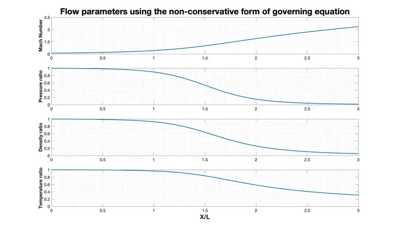
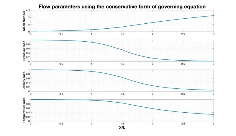
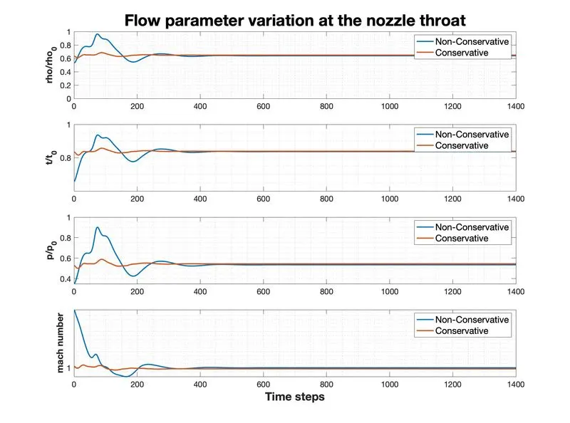
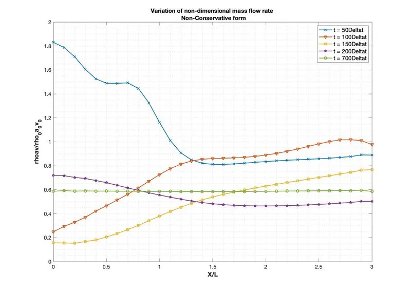
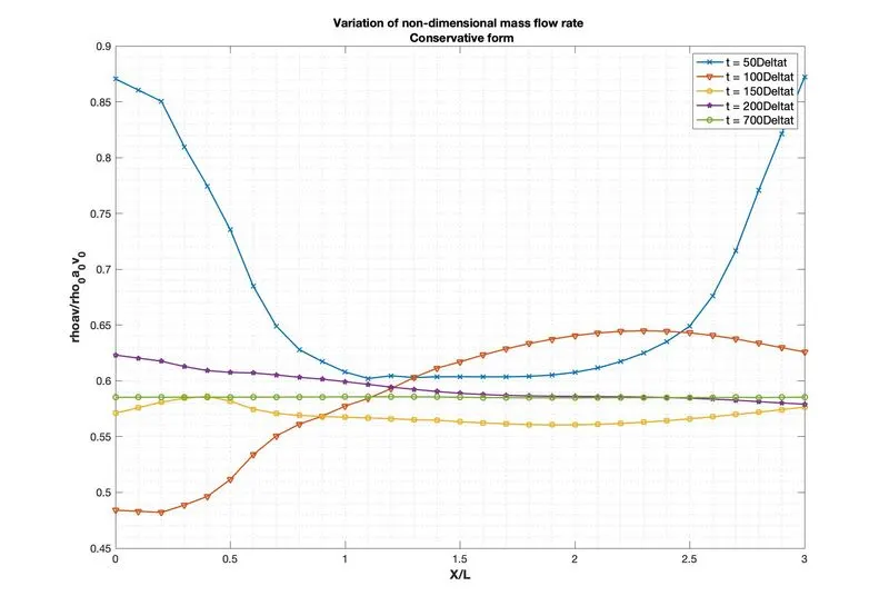
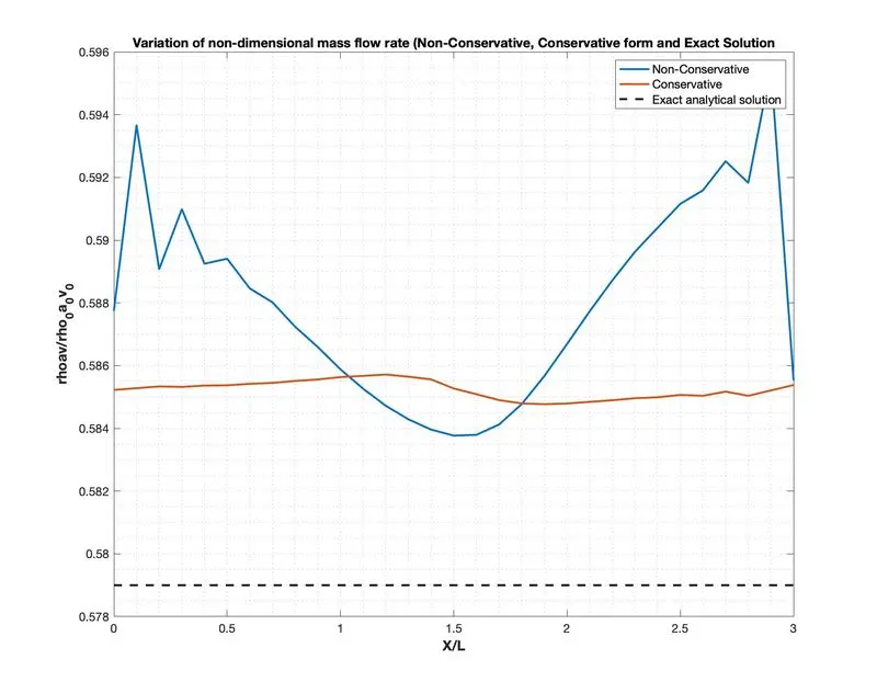
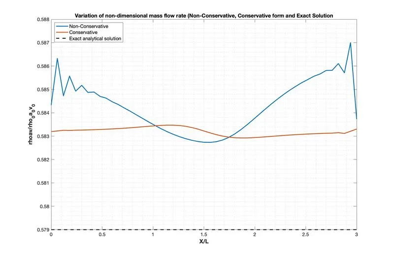
Fig.) Variation of non-dimensional mass flow rate (51 grid points)
Conclusion: -
1. If we look at 'variation of mass flow rate for non-conservative form' and 'variation of mass-flow rate for conservative form' in different time steps, we can see if at smaller time steps the solution is unstable. However, as we increased the time step, the solution become stable. At 700Delta the mass flow rate is stable.
2. As we increased the number of grid points to 51, we can notice that non-conservative form become more stable bur conservative form shows the same behaviour.
3. The conservative form produces an almost constant mass flow rate but the non-conservative form gave highly fluctuating mass flow rate.