Week 5.1 - Mid term project - Solving the steady and unsteady 2D heat conduction problem
Aim: -
Solve 2D steady and unsteady(transient) heat conduction equation.
Objective: -
The problem will be solved using following methods for implicit equations: -
1. Jacobi method
2. Gauss-Seidel method
3. Successive over-relaxation method
The idea is to observe the convergence effect due to these methods. The boundary conditions for the problem are as follows: -
Top Boundary = 600 K
Bottom Boundary = 900 K
Left Boundary = 400 K
Right Boundary = 800 K
Absolute error is 1e-4.
Theory: -
a. Steady state analysis
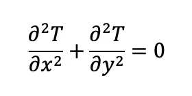
We make use of numerical methods make use of boundary elements. The solutions are obtained at discrete points in our square domain.
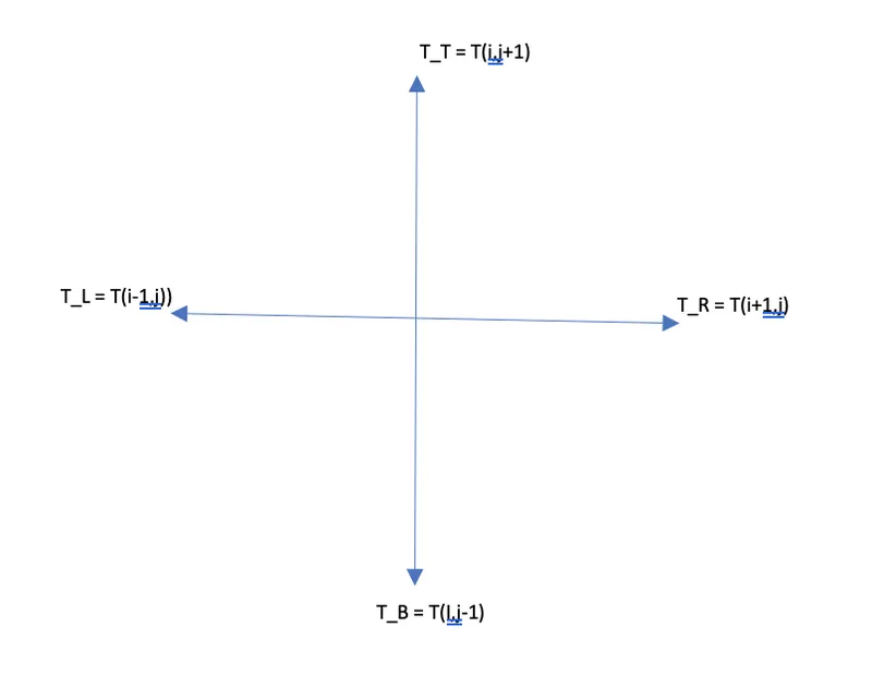
The spacing between the two discrete points in directions x and y are Δx and Δy, respectively. Now we try to formulate the problem,
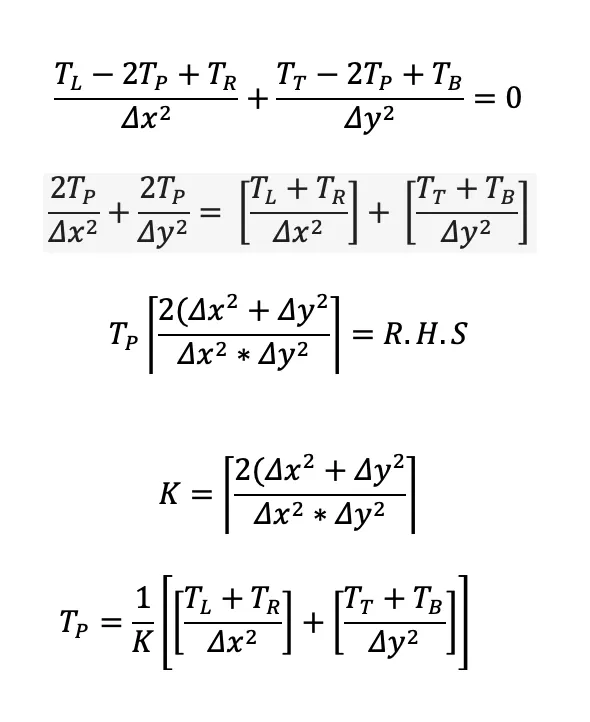
We assume that we have uniform grid spacing.
Results
Results for steady solution: -
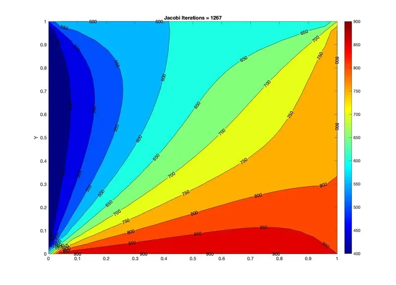
Fig.1) Jacobi Iteration. In solving 2D heat conduction equation using Jacobi method, it takes 214.6471 seconds in 1267 iterations. (number of nodes in x and y directions are 25)
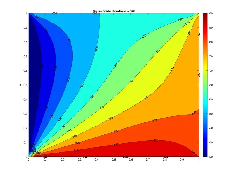
Fig.2) Gauss-Seidel Iteration. In solving 2D heat conduction equation using Gauss-Seidel method, it takes 106.3547 seconds in 676 iterations. (number of nodes in x and y directions are 25)
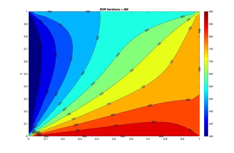
Fig.3) Successive over relaxation. In solving 2D heat conduction equation using SOR method, it takes 68.7575 seconds in 465 iterations. (number of nodes in x and y directions are 25)
MATLAB code for steady state 2D heat conduction: -
clear all
close all
clc

% initial condition
L = 1; % length of domain
nx = 25;
ny = 25;

% mesh generation
x = linspace(0,L,nx);
y = linspace(0,L,ny);
dx = L/(nx-1); % providing grid spacing along the x-axis
dy = L/(ny-1); % providing grid spacing along the y-axis
error = 9e9;
tol = 1e-4;

% assigning BC
T_L = 400;
T_R = 800;
T_T = 600;
T_B = 900;

% Temperature matrix
T = 298*ones(nx,ny)
T(1,:) = T_B
T(end,:) = T_T
T(:,1) = T_L
T(:,end) = T_R

% Edge refining
T(1,1) = (900 + 400)/2;
T(1,end) = (900 + 800)/2;
T(end,1) = (400 + 600)/2;
T(end,end) = (800 + 600)/2;

% Calculation of relaxation factor
% omega = 2/(1+sin(pi*dx));
omega = 1.2;

% Creating a copy of old values
[X,Y] = meshgrid(x,y);
Told = T;

iterative_solver = input('1)Jacobi 2)Gauss Seidel 3) SOR \nEnter an option for the type of solver: ')
k = 2/(dx^2) + 2/(dy^2);

tic
if iterative_solver == 1
    jacobi_iter = 1;
    while(error > tol)
        for i = 2:(nx-1)
            for j = 2:(ny-1)
                term1 = (Told(i-1,j)+Told(i+1,j))/(k*(dx^2));
                term2 = (Told(i,j-1)+Told(i,j+1))/(k*(dy^2));
                T(i,j) = term1 + term2;
            end
        end
        error = max(max(abs(Told-T)));
        Told = T;
        jacobi_iter = jacobi_iter + 1;
        figure(1)
        [A,B] = contourf(X,Y,T)
        set(gca,'YDIR')
        colorbar
        colormap(jet)
        clabel(A,B)
        text = sprintf('Jacobi Iterations = %d',jacobi_iter);
        ylabel('Y')
        title(text)
        pause(0.03)
    end
end

if iterative_solver == 2
    gauss_iter = 1;
    while(error > tol)
        for i = 2:(nx-1)
            for j = 2:(ny-1)
                term1 = (T(i-1,j)+Told(i+1,j))/(k*(dx^2));
                term2 = (T(i,j-1)+Told(i,j+1))/(k*(dy^2));
                T(i,j) = term1 + term2;
            end
        end
        error = max(max(abs(Told-T)));
        Told = T;
        gauss_iter = gauss_iter + 1;
        figure(1)
        [A,B] = contourf(X,Y,T)
        set(gca,'YDIR')
        colorbar
        colormap(jet)
        clabel(A,B)
        text = sprintf('Gauss Seidel Iterations = %d',gauss_iter);
        ylabel('Y')
        title(text)
        pause(0.03)
    end
end

if iterative_solver == 3
    sor_iter = 1;
    while(error > tol)
        for i = 2:(nx-1)
            for j = 2:(ny-1)
                term1 = (T(i-1,j)+Told(i+1,j))/(k*(dx^2));
                term2 = (T(i,j-1)+Told(i,j+1))/(k*(dy^2));
                T(i,j) = (1 - omega)*Told(i,j) + omega*(term1 + term2);
            end
        end
        error = max(max(abs(Told - T)));
        Told = T;
        sor_iter = sor_iter + 1;
        figure(1)
        [A,B] = contourf(X,Y,T)
        set(gca,'YDIR')
        colorbar
        colormap(jet)
        clabel(A,B)
        text = sprintf('SOR Iterations = %d',sor_iter);
        ylabel('Y')
        title(text)
        pause(0.03)
    end
end

Time_taken = toc
b. Unsteady(transient) analysis
In transient(unsteady) heat conduction, the temperature of a body at any points varies with time as well as position in one-dimensional and multi-dimensional systems. This type of heat conductoin is known as transient heat conduction. The 2D heat conduction equation is given by: -
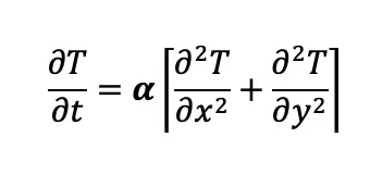
In method of characterisition, we got to know that having a time derivative in the governing equation requires time marching solution.
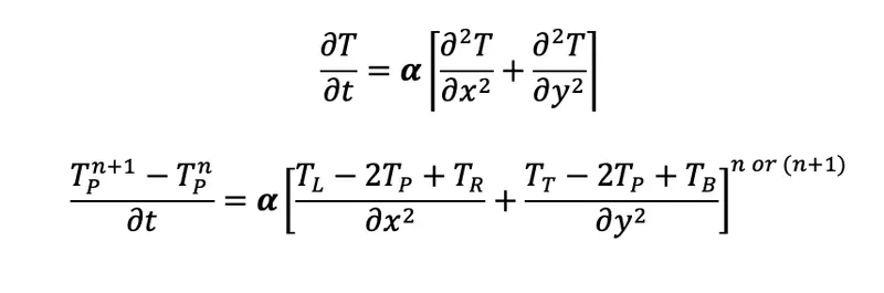
n for explicit scheme
(n+1) for implicit scheme
The final formulas for above schemes are as follow: -

Matlab code for transient 2D heat conduction equation (explicit method): -
clear all
close all
clc

% initial condition
L = 1; % length of domain
nx = 10;
ny = 10;

% mesh generation
x = linspace(0,L,nx);
y = linspace(0,L,ny);
dx = L/(nx-1); % providing grid spacing along the x-axis
dy = L/(ny-1); % providing grid spacing along the y-axis
error = 9e9;
tol = 1e-4;

% assigning BC
T_L = 400;
T_R = 800;
T_T = 600;
T_B = 900;

% defining time
dt = 0.1;
t = 5;
nt = t/dt;

% Temperature matrix
T = 298*ones(nx,ny)
T(1,:) = T_B
T(end,:) = T_T
T(:,1) = T_L
T(:,end) = T_R

% Edge refining
T(1,1) = (900 + 400)/2;
T(1,end) = (900 + 800)/2;
T(end,1) = (400 + 600)/2;
T(end,end) = (800 + 600)/2;

alpha = 1e-3 % convective coefficient
k1 = (alpha*dt)/(dx^2);
k2 = (alpha*dt)/(dy^2);

% Creating a copy of old values
[X,Y] = meshgrid(x,y);
Told = T;

% CFL verification
CFL = k1 + k2;

unsteady_explicit_iter = 1;

tic
for k = 1:nt
    while(error > tol)
        for i = 2:(nx-1)
            for j = 2:(ny-1)
                term1 = Told(i-1,j) - 2*Told(i,j) + Told(i+1,j);
                term2 = Told(i,j-1) - 2*Told(i,j) + Told(i,j+1);
                T(i,j) = Told(i,j) + k1*term1 + k2*term2;
            end
        end
        error = max(max(abs(Told - T)));
        Told = T;
        unsteady_explicit_iter = unsteady_explicit_iter + 1;
        figure(1)
        [A,B] = contourf(X,Y,T)
        set(gca,'YDIR')
        colorbar
        colormap(jet)
        clabel(A,B)
        text = sprintf('Unsteady Explicit Interation = %d',unsteady_explicit_iter);
        ylabel('Y')
        title(text)
        pause(0.03)
    end
end

Time_taken = toc
Result
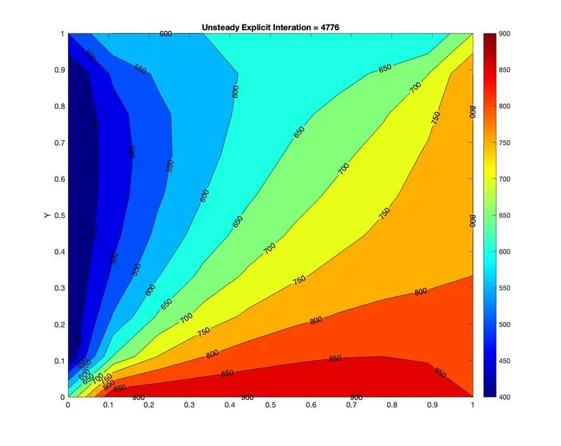
Fig.4) Unsteady Explicit Iteration. In solving unsteady 2D heat conductoin equation, it takes 1.0410e+3 seconds for 4776 iterations. (number of nodes in x and y directions are 10)
Matlab code for transient 2D heat conduction equation (implicit method): -
clear all
close all
clc

% initial condition
L = 1; % length of domain
nx = 10;
ny = 10;

% mesh generation
x = linspace(0,L,nx);
y = linspace(0,L,ny);
dx = L/(nx-1); % providing grid spacing along the x-axis
dy = L/(ny-1); % providing grid spacing along the y-axis
error = 9e9;
tol = 1e-4;

% assigning BC
T_L = 400;
T_R = 800;
T_T = 600;
T_B = 900;

% defining time
dt = 0.001;
%t = 5;
%nt = t/dt;

% Temperature matrix
T = 298*ones(nx,ny);
T(1,:) = T_B
T(end,:) = T_T
T(:,1) = T_L
T(:,end) = T_R

% Edge refining
T(1,1) = (900 + 400)/2;
T(1,end) = (900 + 800)/2;
T(end,1) = (400 + 600)/2;
T(end,end) = (800 + 600)/2;

% Creating a copy of old values
[X,Y] = meshgrid(x,y);
Told = T;
T_prev_dt = T;

alpha = 1.4 % convective coefficient
k1 = (alpha*dt)/(dx^2);
k2 = (alpha*dt)/(dy^2);

% CFL verification
CFL = k1 + k2;

% value of omega
omega = 1.1

iter = 1;

iterative_solver = input('1)Jacobi 2)Gauss Seidel 3) SOR \nEnter an option for the type of solver: ')

tic
for nt = 1:1400
    if iterative_solver == 1

        term1 = (1+2*k1+2*k2)^(-1);
        term2 = k1*term1;
        term3 = k2*term1;

        error = 9e9;
        while(error > tol)
            for i = 2:(nx-1)
                for j = 2:(ny-1)
                    H = Told(i-1,j) + Told(i+1,j);
                    V = Told(i,j-1) + Told(i,j+1);
                    T(i,j) = (T_prev_dt(i,j)*term1) + (H*term2) + (V*term3);
                end
            end
            error = max(max(abs(Told - T)));
            Told = T;
            iter = iter + 1;
        end
    end


    if iterative_solver == 2

        term1 = (1+2*k1+2*k2)^(-1);
        term2 = k1*term1;
        term3 = k2*term1;

        error = 9e9;
        while(error > tol)
            for i = 2:(nx-1)
                for j = 2:(ny-1)
                    H = T(i-1,j) + Told(i+1,j);
                    V = T(i,j-1) + Told(i,j+1);
                    T(i,j) = (T_prev_dt(i,j)*term1) + (H*term2) + (V*term3);
                end
            end
            error = max(max(abs(Told - T)));
            Told = T;
            iter = iter + 1;
        end
    end


    if iterative_solver == 3

        term1 = (1+2*k1+2*k2)^(-1);
        term2 = k1*term1;
        term3 = k2*term1;

        error = 9e9;
        while(error > tol)
            for i = 2:(nx-1)
                for j = 2:(ny-1)
                    H = T(i-1,j) + Told(i+1,j);
                    V = T(i,j-1) + Told(i,j+1);
                    T(i,j) = (1 - omega)*Told(i,j) + omega*((T_prev_dt(i,j)*term1) + (H*term2) + (V*term3));
                end
            end
            error = max(max(abs(Told - T)));
            Told = T;
            iter = iter + 1;
        end
    end
    T_prev_dt = T;
    figure(1)
    [P,Q] = contourf(x,y,T);
    set(gca,'YDIR')
    colorbar;
    colormap(jet);
    clabel(P,Q);
    text = sprintf('Implicit Iterations =  %d',iter)
    ylabel('Y')
    title(text)
    pause(0.03)
end


Time_taken = toc
Results
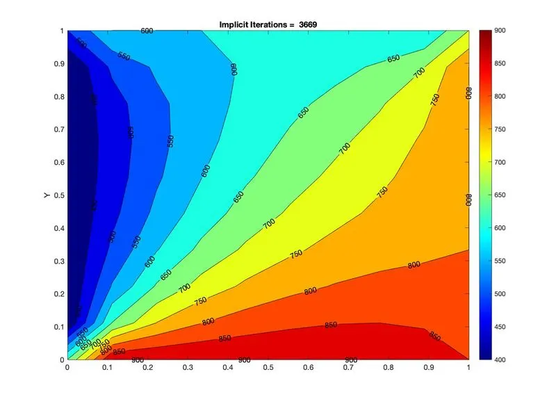
Fig.5) Jacobi unsteady implicit iteration. In solving unsteady 2D heat conductoin equation, it takes 221.092 seconds for 3669 iterations. (number of nodes in x and y directions are 10)
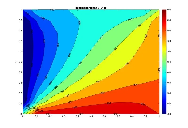
Fig.6) Gauss Seidel unsteady implicit iteration. In solving unsteady 2D heat conductoin equation, it takes 245.2229 seconds for 3115 iterations. (number of nodes in x and y directions are 10)
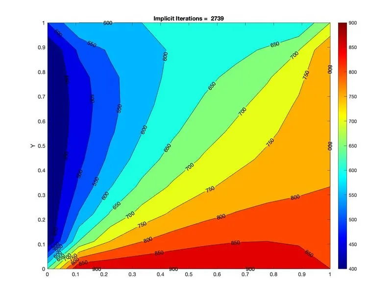
Fig.7) Successive over relaxation unsteady implicit iteration. In solving unsteady 2D heat conductoin equation, it takes 259.4519 seconds for 2739 iterations. (number of nodes in x and y directions are 10)
Conclusion
1. From above figure, it is noticed that successive over relaxation take less iterations than Jacobi and Gauss seidel method. Therefore, the pattern is as follow (Jacobi > Gauss Seidel > Successive over relaxation).
2. From Fig.1,2 and 3, it is noted that time taken by successive over relaxation is less as compared to Jacobi and Gauss Seidel method.
3. Steady state analysis takes less time as compared to unsteady state analysis.