Week 7 - Simulation of a 1D Super-sonic nozzle flow simulation using Macormack Method
Aim: To simulate the isentropic flow for quasi 1D subsonic - supersonic nozzle using conservative and non conservative equations.
Theory :
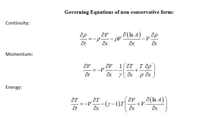
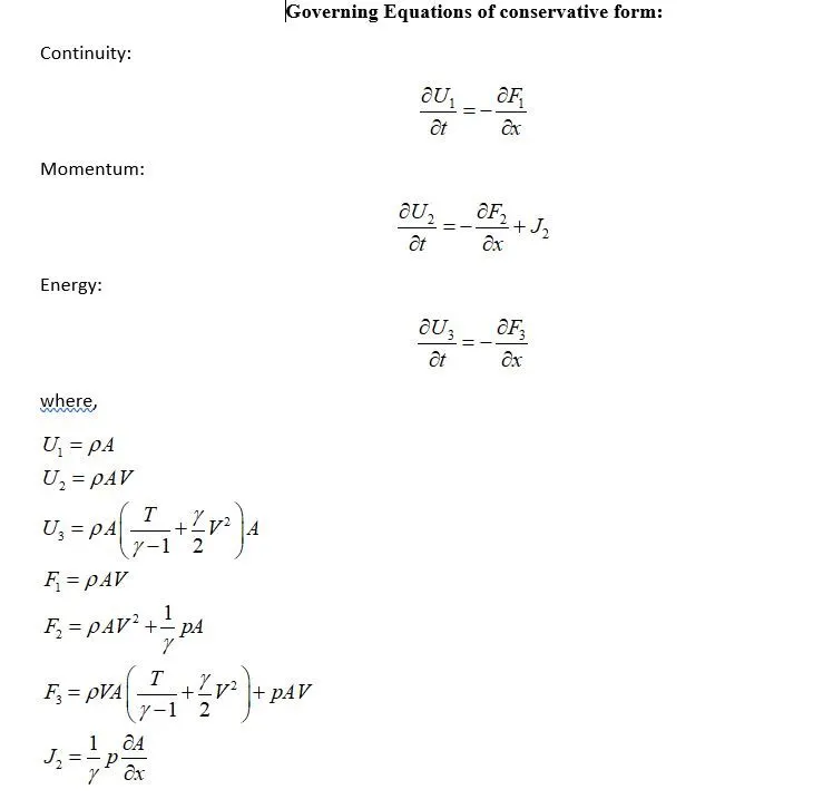
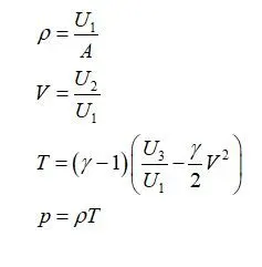
When the air passes through convergent divergent nozzle, its Mach number increases becomes equal to one at the throat and it further increases and becomes greater than one at exit of nozzle. This increase in velocity decreases other parameters like temperature, density, pressure etc. the governing equations are as follows:
Code:
Non - Conservative form:
close all
clear all
clc;

% inputs
n = 31;
x = linspace(0,3,n);
dx = x(2) - x(1);
gamma = 1.4;
C = 0.5;

% calculate profiles
rho = 1 - 0.3146*x;
t = 1 - 0.2314*x;
v = (0.1 + 1.09*x).*t.^0.5;

% area
a = 1 + 2.2*(x-1.5).^2;

% time steps
nt = 1400;

for i=1:n

    time_step(i) = C*(dx/((t(i))^0.5 + v(i)));

end

dt = min(time_step);

% outer time loop
for k = 1:nt

    rho_old = rho;
    v_old = v;
    t_old = t;

    % predictor method
    for j = 2:n-1

        dvdx = (v(j+1) - v(j))/dx;
        drhodx = (rho(j+1) - rho(j))/dx;
        dtdx = (t(j+1) - t(j))/dx;
        dlogadx = (log(a(j+1)) - log(a(j)))/dx;

        % continuity equation
        drhodt_p(j) = -rho(j)*dvdx - rho(j)*v(j)*dlogadx - v(j)*drhodx;

        % momentum equation
        dvdt_p(j) = -v(j)*dvdx - (1/gamma)*(dtdx + (t(j)/rho(j))*drhodx);

        % energy equation
        dtdt_p(j) =  -v(j)*dtdx -(gamma-1)*t(j)*(dvdx + v(j)*dlogadx);

        % solution update
        rho(j) = rho(j) + drhodt_p(j)*dt;
        v(j) = v(j) + dvdt_p(j)*dt;
        t(j) = t(j) + dtdt_p(j)*dt;
    end

    % corrector method
    for j = 2:n-1

        dvdx = (v(j) - v(j-1))/dx;
        drhodx = (rho(j) - rho(j-1))/dx;
        dtdx = (t(j) - t(j-1))/dx;
        dlogadx = (log(a(j)) - log(a(j-1)))/dx;

        % continuity equation
        drhodt_c(j) = -rho(j)*dvdx - rho(j)*v(j)*dlogadx - v(j)*drhodx;

        % momentum equation
        dvdt_c(j) = -v(j)*dvdx - (1/gamma)*(dtdx + (t(j)/rho(j))*drhodx);

        % energy equation
        dtdt_c(j) =  -v(j)*dtdx -(gamma-1)*t(j)*(dvdx + v(j)*dlogadx);


    end

    % compute the average time derivative
    drhodt = 0.5*(drhodt_p + drhodt_c);
    dvdt = 0.5*(dvdt_p + dvdt_c);
    dtdt = 0.5*(dtdt_p + dtdt_c);

    % final solution update
    for i = 2:n-1

        rho(i) = rho_old(i) + drhodt(i)*dt;
        v(i) = v_old(i) + dvdt(i)*dt;
        t(i) = t_old(i) + dtdt(i)*dt;

    end

    % apply the boundary conditions
    %inlet
    v(1) = 2*v(2) - v(3);

    %outlet
    v(n) = 2*v(n-1) - v(n-2);
    rho(n) = 2*rho(n-1) - rho(n-2);
    t(n) = 2*t(n-1) - t(n-2);

    p = rho.*t;
    M = v./t.^0.5;

      m = rho.*a.*v;
%     plot(x,m);
%     xlabel('Length of nozzle');
%     ylabel('Mass flow rate');
%     axis([0 3 0 1.8]);
%     title(sprintf('Time step = %d',k));
%     pause(0.00000000000001);

%     figure(1)
%     subplot(5,1,1)
%     plot(x,M);
%     xlabel('Length of nozzle');
%     ylabel('Mach number');
%     title(sprintf('Time step = %d',k));
%     subplot(5,1,2)
%     plot(x,p);
%     xlabel('Length of nozzle');
%     ylabel('pressure ratio');
%     subplot(5,1,3)
%     plot(x,v);
%     xlabel('Length of nozzle');
%     ylabel('velocity ratio');
%     subplot(5,1,4)
%     plot(x,rho);
%     xlabel('Length of nozzle');
%     ylabel('density ratio');
%     subplot(5,1,5)
%     plot(x,t);
%     xlabel('Length of nozzle');
%     ylabel('Temperature ratio');
%     pause(0.0000001);

end

% figure(2)
subplot(5,1,1)
plot(x,M);
title(sprintf('Steady state solution for Non conservative form at n = %d',n));
xlabel('Length of nozzle');
ylabel('Mach number');
subplot(5,1,2)
plot(x,p);
xlabel('Length of nozzle');
ylabel('pressure ratio');
subplot(5,1,3)
plot(x,v);
xlabel('Length of nozzle');
ylabel('velocity ratio');
subplot(5,1,4)
plot(x,rho);
xlabel('Length of nozzle');
ylabel('density ratio');
subplot(5,1,5)
plot(x,t);
xlabel('Length of nozzle');
ylabel('Temperature ratio');
Conservative form:
close all
clear all
clc;

% inputs
n = 31;
x = linspace(0,3,n);
dx = x(2) - x(1);
gamma = 1.4;
C = 0.5;

% calculate profiles
for i=1:n

    if x(i)>=0 && x(i)<0.5
        rho(i) = 1;
        t(i) = 1;

    elseif x(i)>=0.5 && x(i)< 1.5
        rho(i) = 1 - (0.366*(x(i)-0.5));
        t(i) = 1 - (0.167*(x(i)-0.5));

    else
        rho(i) = 0.634-(0.3879*(x(i) - 1.5));
        t(i) = 0.833 - (0.3507*(x(i) - 1.5));
    end

end

% area
a = 1 + 2.2*(x-1.5).^2;
v = 0.59./(rho.*a);

U1 = rho.*a;
U2 = rho.*a.*v;
U3 = rho.*a.*((t/(gamma-1))+(gamma.*v.^2)/2);
m = rho.*a.*v;

% time steps
nt = 1400;

for j=1:n

    time_step(j) = C*(dx/((t(j))^0.5 + v(j)));

end

dt = min(time_step);

% outer time loop
for k = 1:nt

    U1_old = U1;
    U2_old = U2;
    U3_old = U3;

     F1 = U2;
     F2 = ((U2.^2)./U1)+((gamma-1)/gamma)*(U3-(gamma/2)*((U2.^2)./U1));
     F3 = (gamma.*U2.*U3)./U1 -(gamma*((gamma-1)/2)*(U2.^3)./((U1.^2)));
     %J2 = ((gamma-1)/gamma)*dlogadx*(U3 - (gamma/2)*(U2.^2./U1));

    % predictor method
    for j = 2:n-1

        dadx(j) = (a(j+1) - a(j))/dx;
        J2(j) = (1/gamma)*rho(j)*t(j)*dadx(j);

        dUdt_1_p(j) = - (F1(j+1) - F1(j))/dx;
        dUdt_2_p(j) = - (F2(j+1) - F2(j))/dx + J2(j);
        dUdt_3_p(j) = - (F3(j+1) - F3(j))/dx;

        U1(j) = U1(j) + dUdt_1_p(j)*dt;
        U2(j) = U2(j) + dUdt_2_p(j)*dt;
        U3(j) = U3(j) + dUdt_3_p(j)*dt;

    end

    F1 = U2;
    F2 = ((U2.^2)./U1)+((gamma-1)/gamma)*(U3-(gamma/2)*((U2.^2)./U1));
    F3 = (gamma.*U2.*U3)./U1 -(gamma*((gamma-1)/2)*(U2.^3)./((U1.^2)));
    rho = U1./a;
    v  = U2./U1;
    t  = (gamma-1)*((U3./U1)-((gamma/2)*(v.^2)));

    % corrector method
    for j = 2:n-1

        dadx(j) = (a(j) - a(j-1))/dx;
        J2(j) = (1/gamma)*rho(j)*t(j)*dadx(j);

        dUdt_1_c(j) = - (F1(j) - F1(j-1))/dx;
        dUdt_2_c(j) = - (F2(j) - F2(j-1))/dx + J2(j);
        dUdt_3_c(j) = - (F3(j) - F3(j-1))/dx;

    end

    % compute the average time derivative
    dUdt_1 = 0.5*(dUdt_1_p + dUdt_1_c);
    dUdt_2 = 0.5*(dUdt_2_p + dUdt_2_c);
    dUdt_3 = 0.5*(dUdt_3_p + dUdt_3_c);

    % final solution update
    for i = 2:n-1

        U1(i) = U1_old(i) + dUdt_1(i)*dt;
        U2(i) = U2_old(i) + dUdt_2(i)*dt;
        U3(i) = U3_old(i) + dUdt_3(i)*dt;

        rho(j) = U1(j)/a(j);
        v(j) = U2(j)/U1(j);
        t(j) = (gamma-1)*(U3(j)/U1(j) - (gamma/2*(v(j))^2));

    end

    % apply the boundary conditions
    %inlet
    U1(1) = a(1);
    U2(1) = 2*U2(2) - U2(3);
    v(1) = U2(1)/U1(1);
    U3(1) = U1(1)*((t(1)/(gamma-1))+((gamma/2)*v(1)^2));

    %outlet
    U1(n) = 2*U1(n-1) - U1(n-2);
    U2(n) = 2*U2(n-1) - U2(n-2);
    U3(n) = 2*U3(n-1) - U3(n-2);

    p = rho.*t;
    M = v./t.^0.5;

    m = rho.*a.*v;
%     plot(x,m);
%     xlabel('Length of nozzle');
%     ylabel('Mass flow rate');
%     axis([0 3 0 1.8]);
%     title(sprintf('Time step = %d',k));
%     pause(0.00000000000001);

%     figure(1)
%     subplot(5,1,1)
%     plot(x,M);
%     xlabel('Length of nozzle');
%     ylabel('Mach number');
%     title(sprintf('Time step = %d',k));
%     subplot(5,1,2)
%     plot(x,p);
%     xlabel('Length of nozzle');
%     ylabel('pressure ratio');
%     subplot(5,1,3)
%     plot(x,v);
%     xlabel('Length of nozzle');
%     ylabel('velocity ratio');
%     subplot(5,1,4)
%     plot(x,rho);
%     xlabel('Length of nozzle');
%     ylabel('density ratio');
%     subplot(5,1,5)
%     plot(x,t);
%     xlabel('Length of nozzle');
%     ylabel('Temperature ratio');
%     pause(0.000000000001);

end

%figure(2)
subplot(5,1,1)
plot(x,M);
title(sprintf('Steady state solution for conservative form at n = %d',n));
xlabel('Length of nozzle');
ylabel('Mach number');
subplot(5,1,2)
plot(x,p);
xlabel('Length of nozzle');
ylabel('pressure ratio');
subplot(5,1,3)
plot(x,v);
xlabel('Length of nozzle');
ylabel('velocity ratio');
subplot(5,1,4)
plot(x,rho);
xlabel('Length of nozzle');
ylabel('density ratio');
subplot(5,1,5)
plot(x,t);
xlabel('Length of nozzle');
ylabel('Temperature ratio');
Result:
Non conservative form:
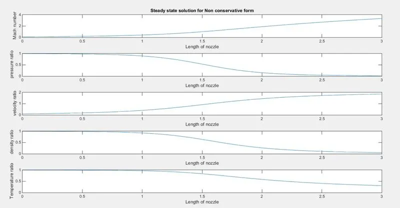
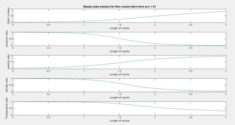
The non conservative form shows the distribution of Mach number, pressure ratio, velocity ratio, density ratio and temperature ratio inside the convergent divergent nozzle. It is clear from the graph that Mach number is increasing while pressure ratio, density ratio, temperature ratio is decreasing.
Time wise variation:
mass flow rate:
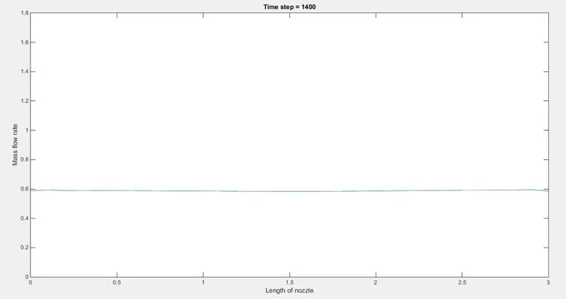
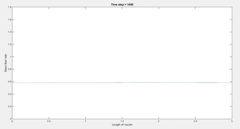
The mass flow rate initially varies but later it becomes constant throughout the nozzle. The graph shows time wise variation of mass flow rate.
Grid independent test:
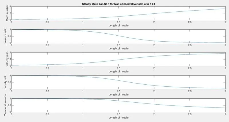
Grid independent test is carried out by chaging the number of nodes in length of nozzle. Initially it is kept 31 then 41 and the 61. All shows the same result. It shows the results are independent of grid size.
Conservative Form:
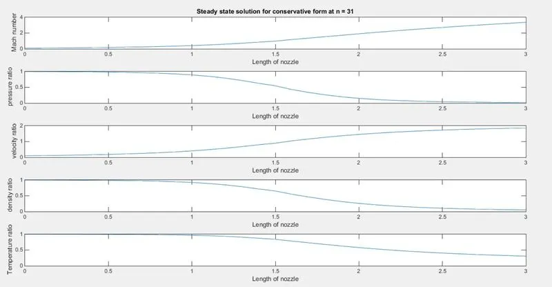
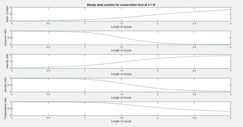
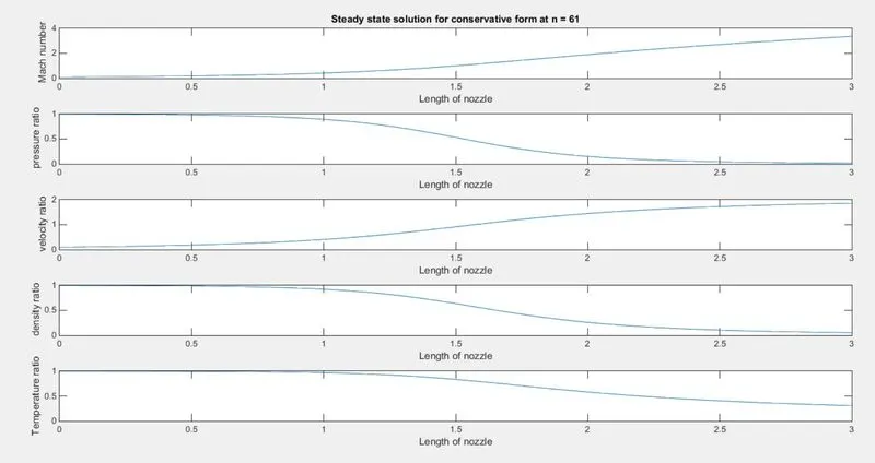
The results of conservative form are very much similar to non conservative form. The mach number and velocity is increasing with length while other parameters like temperature, density, pressure is decreasing.
Time wise variation:
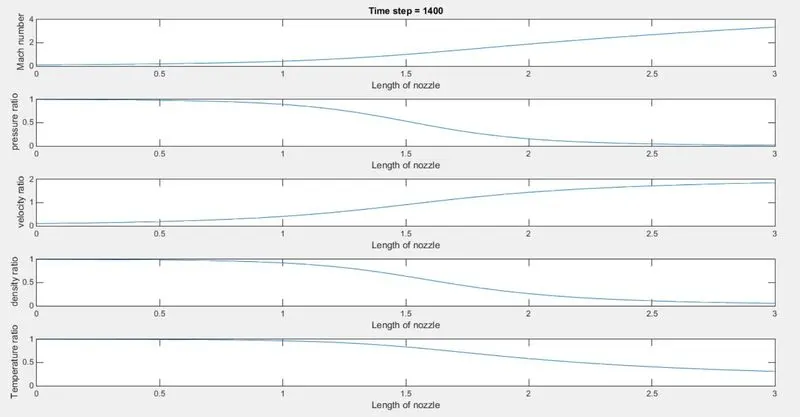
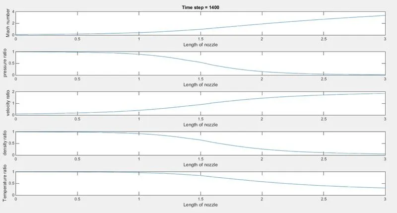
This graph shows the steady state achived after 1400 time steps.
Mass flow rate:
mass flow rate becomes steady after 1400 time steps.
Grid independent test:
The grid independent test is done by changing the grid size of the length of nozzle. The results for n = 31, 41 and 61 are almost same. It means grid size of 31 elements is good for simulation.
Comparison of mass flow rate of conservative and non conservative equations:
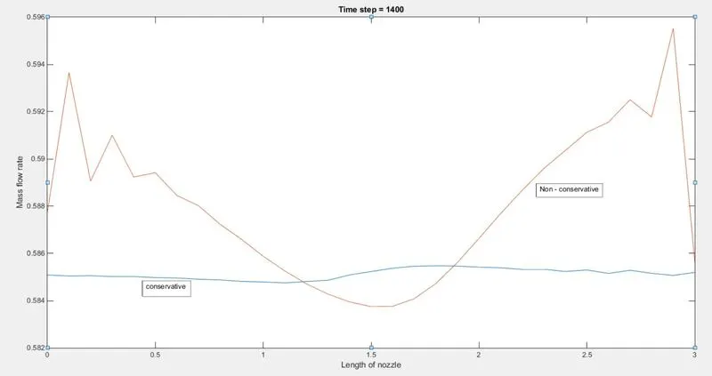
The comparison shows that the conservative form mass flow rate is more closer towards exact results and also it is more stable. While the non conservative form mass flow rate is even after achieving steady state is still having some deviations. This proves for mass flow rate conservation form of equations work better than non conservative form.