Week 3.5 - Deriving 4th order approximation of a 2nd order derivative using Taylor Table method

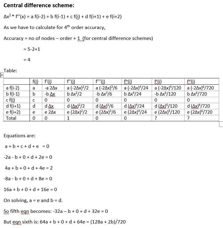
Central difference scheme:

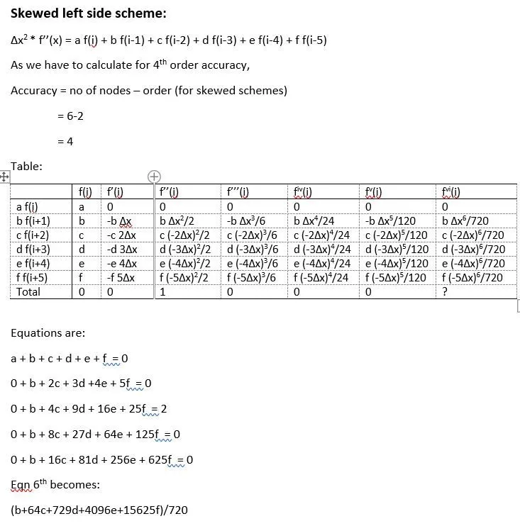
left side scheme:

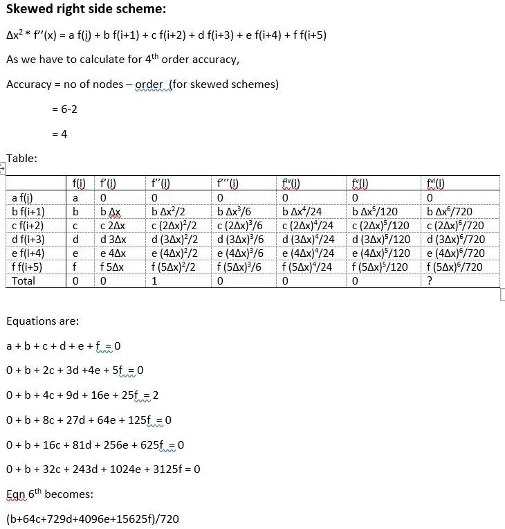
right side scheme:

comparison of 3 schemes in matlab program:

close all
clear all
clc

x = pi/3;
dx = linspace(0.001,0.1,1000);

%exact solution
y = -2*exp(x)*sin(x);

a_cd = [1 1 1 1 1;-2 -1 0 1 2;4 1 0 1 4;-8 -1 0 1 8;16 1 0 1 16];

b_cd = sym(inv(a_cd));

c_cd = b_cd*[0;0;2;0;0];

a_ls = [1 1 1 1 1 1;0 1 2 3 4 5;0 1 4 9 16 25;0 1 8 27 64 125;0 1 16 81 256 625;0 1 32 243 1024 3125];

b_ls = sym(inv(a_ls));

c_ls = b_ls*[0;0;2;0;0;0];

a_rs = [1 1 1 1 1 1;0 1 2 3 4 5;0 1 4 9 16 25;0 1 8 27 64 125;0 1 16 81 256 625;0 1 32 243 1024 3125];

b_rs = sym(inv(a_rs));

c_rs = b_rs*[0;0;2;0;0;0];

for i=1:1000

    % solving through central difference

    y_cd(i) = (c_cd(1)*(exp(x-2*dx(i))*cos(x-2*dx(i))) + c_cd(2)*(exp(x-dx(i))*cos(x-dx(i))) + c_cd(3)*(exp(x)*cos(x)) + c_cd(4)*(exp(x+dx(i))*cos(x+dx(i))) + c_cd(5)*(exp(x+2*dx(i))*cos(x+2*dx(i))))/dx(i)^2;

    error_cd(i) = abs(y_cd(i) - y);
    
    % solving using left side skewed 

    y_ls(i) = (c_ls(1)*(exp(x)*cos(x)) + c_ls(2)*(exp(x-dx(i))*cos(x-dx(i))) + c_ls(3)*(exp(x-2*dx(i))*cos(x-2*dx(i))) + c_ls(4)*(exp(x-3*dx(i))*cos(x-3*dx(i))) + c_ls(5)*(exp(x-4*dx(i))*cos(x-4*dx(i))) + c_ls(6)*(exp(x-5*dx(i))*cos(x-5*dx(i))))/dx(i)^2;
    
    error_ls(i) = abs(y_ls(i) - y);
    
    % solving using right side skewed 

    y_rs(i) = (c_rs(1)*(exp(x)*cos(x)) + c_rs(2)*(exp(x+dx(i))*cos(x+dx(i))) + c_rs(3)*(exp(x+2*dx(i))*cos(x+2*dx(i))) + c_rs(4)*(exp(x+3*dx(i))*cos(x+3*dx(i))) + c_rs(5)*(exp(x+4*dx(i))*cos(x+4*dx(i))) + c_rs(6)*(exp(x+5*dx(i))*cos(x+5*dx(i))))/dx(i)^2;
    
    error_rs(i) = abs(y_rs(i) - y);


end

loglog(dx,error_cd);
hold on
loglog(dx,error_rs);
hold on
loglog(dx,error_ls);
legend('central difference','right side','left side');
ylabel('error');
xlabel('dx');


 

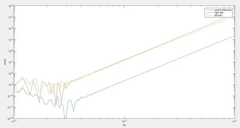
the graph are as follows:

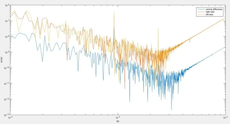
explaination of the problem:

The fourth order approximation for the second order derivative has been derived using central difference, left side skewed and right side skewed schemes. The code has been written for solving e^x*cos(x).

the results show that the central difference scheme is more stable and has very less amount of errrors as compared to skewed righ or left side.

however, when dx becomes smaller, at certain points left or right side scheme error becomes less than central difference schemes.

Though it is clear that central difference is much better than right or left side scheme but at boundary position we have to use one side skewed scheme (right or left). Central difference scheme uses both forward and backward nodes, but at the boundary nodes we have either left or right nodes. So here left side or right side skewed scheme becomes useful. If we want to calculate the parameter at left boundary than right side scheme can be used and if we want to calculate at right boundary then left side scheme can be used. For in-between points we can use central difference scheme.