Week 7 - Simulation of a 1D Super-sonic nozzle flow simulation using Macormack Method
Objectives
1. To derive both the conservation and non-conservation forms of 1d super nozzle.
2.to sovle them using the MacCormack's technique.
3. To determine steady-state temperature distribution for the flow-field variables and to investigate the difference between the two forms of governing equations by comparing their solutions.
4. And to plot steady-state distribution of primitive variables inside the nozzle.
5. To plot Time-wise variation of the primitive variables
6.Variation of Mass flow rate distribution inside the nozzle at different time steps during the time-marching process
7. And to Compare Normalized mass flow rate distributions of both forms.
Theroy
l
We consider the steady, isentropic flow through a convergent-divergent nozzl_e as sketched in Fig. 7 .1. The flow at the inlet to the nozzle comes from a reservoir where the pressure and temperature are denoted by p0 , and To, respectively. The cross-sectional areaofthe reservoir is large ( theoretically, A --+ oo ), and hence thevelocity is very small ( V --+ O). Thus, Po and T0 are the stagnatio~ values,_ or totalpressure and total temperature, respectively. The flow expands 1sentrop1cally. tosupersonic speeds at the nozzle exit, where the exit pressure, temperature, velocity,and Mach number are denoted by Pe, Te, V.,, and Me, respectlvely. The flow locally subsonic in the convergent section if the nozzle, sonic at the throat (minimum area), and supersonic at the divergent section. The sonic flow(M = 1) at the throat means that the local velocity at this location 1s equal to
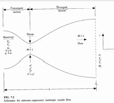
the local speed of sound. Using an asterisk to denote sonic flow values, we have atthe throat V = V* = a*. Similarly, the sonic flow values of pressure and temperatureare denoted by p* and T*, respectively. The area of the sonic throat is denoted byA*. We assume that at a given section, where the cross-sectional area is A, the flowproperties are uniform across that section. Hence, although the area of the nozzlechanges as a function of distance along the nozzle, x, and therefore in reality theow field is two-dimensional (theflow varies in.the two-dimensional .ry space), wemake the assumption that the flow properties-vary only with x; this is tantamount toassuming uniform flow properties across any given cross section. Such flow isdefined as quasi-one-dimensional fl.ow.
The governing continuity, momentum, and energy equations for this quasione-dimensional, steady, isentropic flow can be expressed, respectively, as
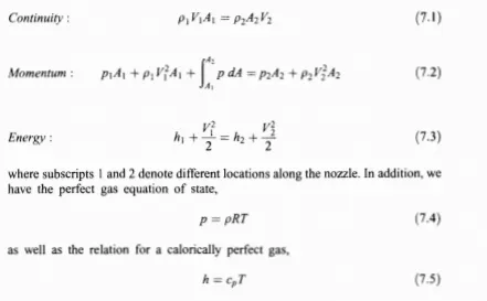
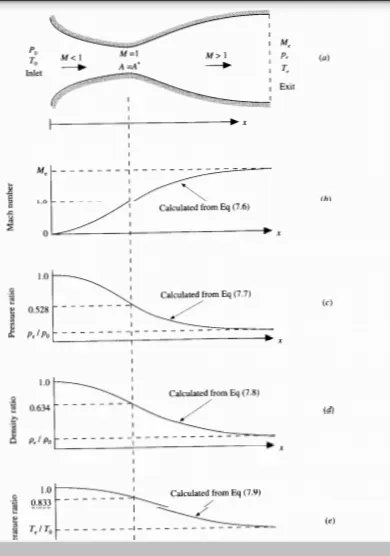
Equations (7.1) to (7.5) can be solved analytically for the flow throughthe nozzle. Some results are as follows. The Mach number variation throughthe nozzle is governed exclusively by the area ratio A/A* through the relation

where y = ratio of specific heats = cplcv. For air at standard conditions, y = 1.4. Fora nozzle where A is specified as a function of x, hence A/A* is known as a functionof x, then Eq. (7.6) allows the (implicit) calculation of Mas a function of x. This issketched in Fig. 7.2b. In turn, the variation of pressure, density, and temperature as afunction of Mach number ( and hence as a function of Al A*, thus x) is given,
CFD SLOUTION
THE SET UP
1. The governing flow equations will be couched in terms of partial differentialequations suitable for the time-marching solution of quasi-one-dimensional flow(the closed-form algebraic equations discussed in Sec. 7.2 are for a steady flowand are not suitable for the present purpose).
2. The finite-difference expressions pertaining to MacCormack's technique asapplied to this problem will be set up.
3. Other details for the numerical solution (such as the calculation of the time stepand the treatment of boundary conditions) will be formulated.
THE GOVERNING EQUATION can be dervied in two forms such as consevative form and non conservative form
1.NON CONSEVATIVE FORM-the governing equation are
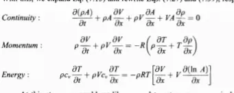
At this stage, we could readily proceed to set up our numerical solution ofEqs. (7.42) to (7.44). Note that these are written in terms of dimensional variables.This is fine, and many CFD solutions are carried out directly in terms of sucdimensional variables. Indeed, this has an added engineering advantage because itgives you a feeling for the magnitudes of the real physical quantities as the solutionprogresses. However, for nozzle flows, the flow-field variables are frequentlyexpressed in terms of nondimensional variables, such as those sketched in Fig.7.2, where the flow variables are referenced to their reservoir values. Thenondimensional variables p/p0 , p/p0 , and TIT0 vary between O and I, whichis an "aesthetic" advantage when presenting the results. Because fluiddynamicistsdealing with nozzle flows so frequently use these nondimensional terms, we willollow suit here. (A number of CFD practitioners prefer to always deal withnondimensional variables, whereas others prefer dimensional variables; as far as thenumerics are concerned, there should be no real difference, and the choice is really amatter of your personal preference.) Therefore, returning to Fig. 7.1, where the
reservoir temperature and density are denoted by To and p0 , respectively, we definethe nondimensional temperature and density, respectively, as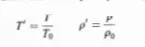
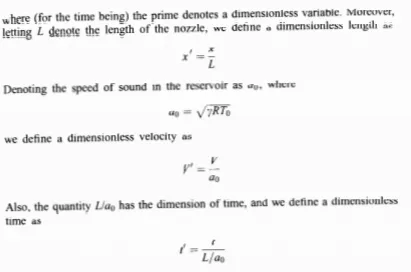
Returning to Eq. (7.42) and introducing the nondimensional variables, we
have



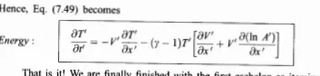
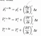
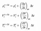
next we apply forward differncing for the space variables



next we calculate flow variables
next we corrected values where we apply the reverse difference for space variables
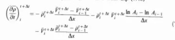
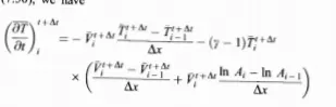
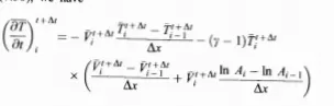
next we calculate the average values
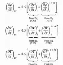
we calculate flow variables
and the code is as follows
n=31
x=linspace(0,3,n)
dx=x(2)-x(1)
n=31
l=3
C=0.5
nt=1400
gamma=1.4
tic
[rho,t,v,p,M,flow_rate_n]=non_conseravtive(l,n,C,dx,nt)
toc
time_non=toc
tic
[rhoc,tc,vc,pc,mc,flow_ratec]=conseravtive(l,n,C,dx,nt)
toc
time_con=toc
fprintf('time_of excuation for  conseravative=%0.4gs',time_con)
figure(7)
plot(x,flow_rate_n,'b','linewidth',2)
hold on
plot(x,flow_ratec,'r','linewidth',2)
title('comparsion of flow variables for conservative form and non conservative form')
legend('conseravative','nonconseravative')
grid on
function[rho,t,v,p,M,flow_rate_n]=non_conseravtive(l,n,C,dx,nt)
x=linspace(0,3,n)
gamma=1.4
throat=(n+1)/2
rho=1-(0.3146.*x);
t=1-(0.2314*x)
v=(0.1+(1.09.*x).*(t.^0.5))
a=1+(2.2*((x-1.5).^2))


flow_rate_old=0

t_arary=(1:nt)
dt=0.0201
for m=1:n
    dt_x(m)=(C*dx)/((t(i)).^0.5+v(i))
end
 dt=min(dt_x)
for k=1:nt
    rho_old=rho
    v_old=v
    t_old=t
    for j=2:n-1
        dvdx=(v(j+1)-v(j))/dx
        drhodx=(rho(j+1)-rho(j))/dx
        dtdx=(t(j+1)-t(j))/dx
       dadx=(log(a(j+1))-log(a(j)))/dx
        drho_dt_p(j)=-rho(j)*dvdx-rho(j)*v(j)*dadx-v(j)*drhodx
        dv_dt_p(j)=-v(j)*dvdx-(1/gamma)*(dtdx+(t(j)/rho(j))*drhodx)
        dt_dt_p(j)=-v(j)*dtdx-(gamma-1)*t(j)*(dvdx+v(j)*dadx)
   rho(j)=rho_old(j)+drho_dt_p(j)*dt
    v(j)=v_old(j)+dv_dt_p(j)*dt
    t(j)=t_old(j)+dt_dt_p(j)*dt


    end

for j=2:n-1
 dvdx=(v(j)-v(j-1))/dx
        drhodx=(rho(j)-rho(j-1))/dx
        dtdx=(t(j)-t(j-1))/dx
       dadx=(log(a(j))-log(a(j-1)))/dx
        drho_dt_c(j)=-rho(j)*dvdx-rho(j)*v(j)*dadx-v(j)*drhodx
        dv_dt_c(j)=-v(j)*dvdx-(1/gamma)*(dtdx+(t(j)/rho(j))*drhodx)
        dt_dt_c(j)=-v(j)*dtdx-(gamma-1)*t(j)*(dvdx+v(j)*dadx )
end
rho_avg=0.5.*(drho_dt_p+drho_dt_c)
v_avg=0.5.*(dv_dt_p+dv_dt_c)
t_avg=0.5.*(dt_dt_p+dt_dt_c)
for i=2:n-1
    rho(i)=rho_old(i)+rho_avg(i)*dt
    v(i)=v_old(i)+v_avg(i)*dt
    t(i)=t_old(i)+t_avg(i)*dt
end
v(1)=2*v(2)-v(3)
v(n)=2*v(n-1)-v(n-2)
rho(n)=2*rho(n-1)-rho(n-2)
t(n)=2*t(n-1)-t(n-2)
p=rho.*t
M=v./(t.^.5)
flow_rate_n=rho.*v.*a
rho_throat(k)=rho(throat)
t_throat(k)=t(throat)
p_throat(k)=p(throat)
M_throat(k)=M(throat)
flow_rate_throat(k)=flow_rate_n(throat)
figure(1)
title('flow rates for at different instant of times for non conservative for 31 grid points')
legend('flow rates at delta t')
hold on
if k==50
plot(x,flow_rate_n,'r','linewidth',2)
grid on

else if k==100
    plot(x,flow_rate_n,'g','linewidth',2)
grid on

else if k==200
        plot(x,flow_rate_n,'y','linewidth',2)
   grid on

else if k==500
            plot(x,flow_rate_n,'b','linewidth',2)
       grid on

    else if k==700
                plot(x,flow_rate_n,'b','linewidth',2)
               grid on

end
end

end
end


end
legend('50 deltat','100deltat','200deltat','500deltat','700deltat')
xlabel('x/l')
ylabel('rhova/rho_{0}v_{0}a{0}')
end
figure(2)

subplot(5,1,1)
plot(x,v,'r','linewidth',2)
title(' flow variables for 1d supper nozzle  for non conseravative for 31 grid points')
legend('velocity')
grid on
xlabel('x values')
ylabel('velocity')
subplot(5,1,2)
plot(x,M,'b','linewidth',2)
grid on
xlabel('xvalues')
ylabel('mach number')
legend('mach number')
grid on
subplot(5,2,3)
plot(x,rho,'y','linewidth',2)
legend('density')
grid on
xlabel('xvalues')
ylabel('rho')
subplot(5,2,4)
grid on
plot(x,t,'b')
legend('temperature')
grid on
xlabel('xvalues')
ylabel('temperature')
subplot(5,2,5)
plot(x,p,'b','linewidth',2)
legend('pressure')
grid on
xlabel('xvalues')
ylabel('pressure')

figure(3)

subplot(4,1,1)

plot(1:nt,rho_throat)
title('time variation  of flow varibles for non conserative form for 31 grid points')
legend('density')
grid on
ylabel('rho')
subplot(4,1,2)
plot(1:nt,t_throat,'linewidth',2)
legend('temperature')
grid on
ylabel('temerature')
subplot(4,1,3)
plot(1:nt,p_throat,'linewidth',2)
legend('pressure')
grid on
ylabel('pressure')
subplot(4,1,4)
plot(1:nt,M_throat,'linewidth',2)
legend('mach number')
grid on
ylabel('mach number')

end
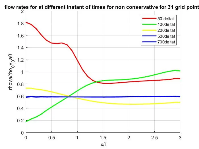
figure(1);flow rate at different instant of time for 31 grid points for non conservative form
from the above graph we can conclude that mass flow rate attains stablity after 700 time step for nonconservative form i,e the mass conserved after 500th time step.
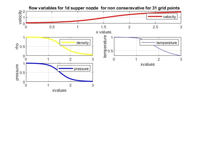
figure(2):flow variables for non consrevartive form for 31 grid points
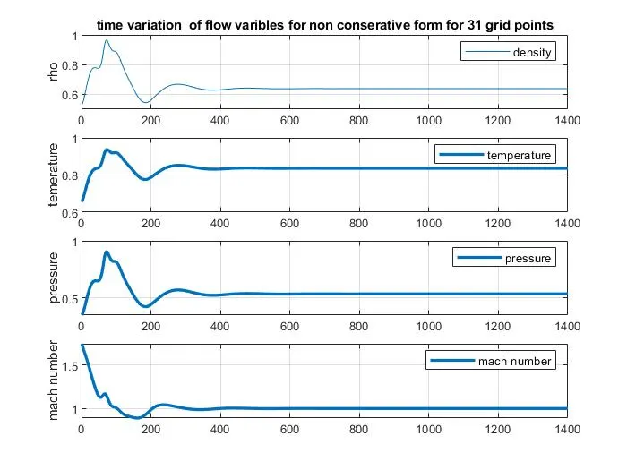
figure(3):flow variables at different instant of time for non conservative form for 31 grid points
for 61 grid points we have following graphs
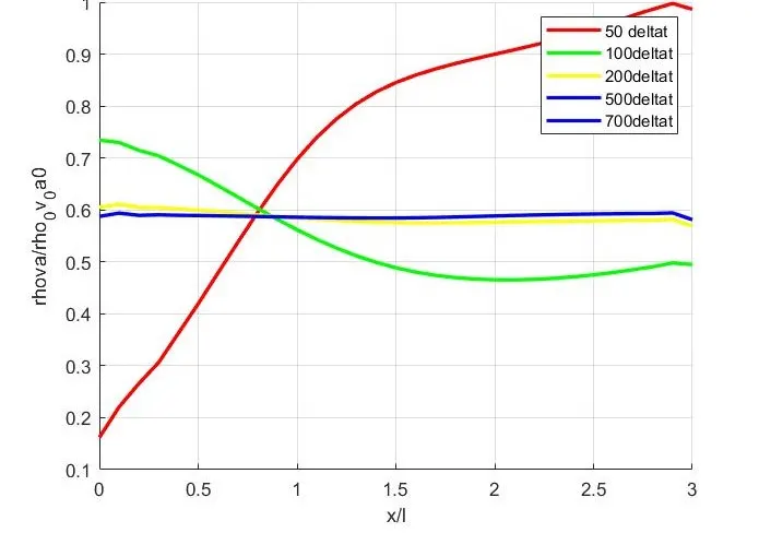
figure(4):flow rate at different instant of time for 61 grid points for non conservative form
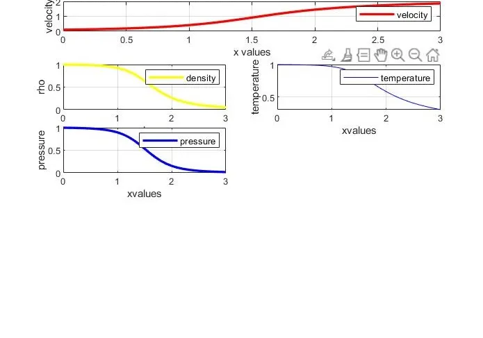
figure(5) flow variables for non conservative for 61 grid points
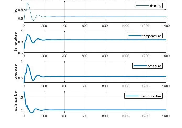
figure(6) :time varition of the fluid variables for 61 grid points for non conseravtive form
theroy for the conservative form
we divide the conservative equation in to flux vector,sloution vector and souurce term
nad we have equqtions ha
u1=rho*area
u2=rho*area*velocity
u3=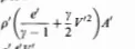
and we have flux vector and the sloution term as
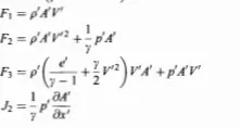
and the above equation is written as
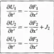
from u1,u2 and u3 we can caluclate fluid variables as
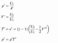
for corrector step we use the u1 ,u2 and u3 from predicted values and we apply the reverse difference.
and the code is as follows
function[rhoc,tc,vc,pc,mc,flow_ratec]=conseravtive(l,n,C,dx,nt)
x=linspace(0,3,n);
u2=0.59


gamma=1.40;

for i=1:length(x)
if x(i)>=0 && x(i)<=0.5;
    rho_int(i)=1;
    t_int(i)=1;
elseif x(i)>=0.5 &&x(i)<=1.5
    rho_int(i)=1-0.366*(x(i)-0.56);
    t_int(i)=1-0.167*(x(i)-0.5);
elseif x(i)>=1.5 && x(i)<=3.5
    rho_int(i)=0.634-0.3879*(x(i)-1.5);
    t_int(i)=0.833-0.3507*(x(i)-1.5);
end
end
rhoc=rho_int
tc=t_int
a=1+(2.2*((x-1.5).^2));

v=u2./((rho_int.*a));
vc=v
   u1=rhoc.*a;
   u2=rhoc.*a.*vc;
   u3=rhoc.*a.*((tc/(gamma-1))+(0.5*gamma.*vc.^2));


pc=rhoc.*tc;
   mc=vc./(sqrt(tc));
for m=1:n
    dt_x(m)=(C*dx)/((t(i)).^0.5+v(i))
end
 dt=min(dt_x)


throat=(n+1)/2;
t_array=(1:nt)
for j=1:nt
   u1_old=u1;
   u2_old=u2;
   u3_old=u3;
   f1=u2;
   f2=((u2.^2)./u1)+((gamma-1)/gamma).*(u3-((gamma/2)*(u2.^2./u1)));
   f3=((gamma.*u2.*u3)./u1)-((gamma*(gamma-1))/2)*(u2.^3)./(u1.^2);
   for m=2:n-1

       j2(m)=(1/gamma)*(rhoc(m)*tc(m))*((a(m+1)-a(m))/dx)
       du1dt_p(m)=-(f1(m+1)-f1(m))/dx;
       du2dt_p(m)=-((f2(m+1)-f2(m))./dx)+j2(m);
       du3dt_p(m)=-(f3(m+1)-f3(m))./dx;
       u1(m)=(u1_old(m)+(du1dt_p(m).*dt));
       u2(m)=(u2_old(m)+(du2dt_p(m).*dt));
       u3(m)=(u3_old(m)+( du3dt_p(m).*dt));
       rhoc(m)=u1(m)./a(m);
       vc(m)=(u2(m)./u1(m));
       tc(m)=(gamma-1).*((u3(m)./u1(m))-(gamma./2).*((u2(m)./u1(m)).^2));
   pc=rhoc(m).*tc(m);
   end
   f1=u2;
   f2=((u2.^2)./u1)+((gamma-1)./gamma).*(u3-(gamma./2).*((u2).^2./u1));
   f3=((gamma.*u2.*u3)./u1)-((gamma.*(gamma-1))./2).*((u2.^3)./(u1.^2)) ;
for e=2:n-1

       j2(e)=(1/gamma)*rhoc(e)*tc(e)*((a(e)-a(e-1))/dx)
       du1dt_c(e)=-(f1(e)-f1(e-1))./dx;
       du2dt_c(e)=-((f2(e)-f2(e-1))./dx)+j2(e);
       du3dt_c(e)=-(f3(e)-f3(e-1))./dx;
end
       du1dt_av=0.5.*(du1dt_p+du1dt_c);
       du2dt_av=0.5.*(du2dt_p+du2dt_c);
       du3dt_av=0.5.*(du3dt_p+du3dt_c);
       for b=2:n-1
           u1(b)=(u1_old(b)+(du1dt_av(b).*dt));
           u2(b)=(u2_old(b)+(du2dt_av(b).*dt));
           u3(b)=(u3_old(b)+(du3dt_av(b).*dt));
       end

       u1(1)=a(1)*rhoc(1);
   u2(1)=2*u2(2)-u2(3);
   vc(1)=u2(1)./u1(1)
   u3(1)=u1(1)*((tc(1)/(gamma-1))+((0.5*gamma)*(vc(1)).^2));
   u1(n)=2*u1(n-1)-u1(n-2);
   u2(n)=2*u2(n-1)-u2(n-2);
   u3(n)=2*u3(n-1)-u3(n-1);
    rhoc=u1./a
       vc=(u2./u1);
       tc=(gamma-1).*((u3./u1)-(gamma./2).*((u2./u1).^2))
   pc=rhoc.*tc;
   flow_ratec=rhoc.*a.*vc;
   mc=vc./(sqrt(tc));

   rho_throat(j)=rhoc(throat);
t_throat(j)=tc(throat);
p_throat(j)=pc(throat);
m_throat(j)=mc(throat);
flow_rate_throat(j)=flow_ratec(throat);
mass2=figure(4)
hold on
title('flow rates at different instant of time for conserative form for 31 grid points')
if j==50
plot(x,flow_ratec,'r','linewidth',2);

grid on
else if j==100
    plot(x,flow_ratec,'b','linewidth',2);

    grid on
else if j==200
        plot(x,flow_ratec,'y','linewidth',2);

   grid on
else if j==500
            plot(x,flow_ratec,'g','linewidth',2);

       grid on
    else if j==700
                plot(x,flow_ratec,'b','linewidth',2);

                grid on

end
end

end
end
end
legend('50 deltat','100deltat','200deltat','500deltat','700deltat')
xlabel('x/l')
ylabel('rhova/rho_{0}v_{0}a{0}')
end
figure(5)

subplot(5,1,1)
grid on
plot(x,vc,'r','linewidth',2);
title('flow variables for 1d nozzle for consrvative form for 31 grid points')
xlabel('x values')
ylabel('velovity')
legend('velocity')
grid on
subplot(5,1,2)
plot(x,mc,'b','linewidth',2);
xlabel('xvalues')
ylabel('mach number')
legend('mach number')
grid  on
subplot(5,2,3)
plot(x,rhoc,'y','linewidth',2);
xlabel('xvalues')
ylabel('rho')
legend('density')
grid on
subplot(5,2,4)
plot(x,tc,'b','linewidth',2);
xlabel('xvalues')
ylabel('temperature')
legend('temperature')
grid on
subplot(5,2,5)
plot(x,pc,'b','linewidth',2)
legend('pressure');
xlabel('xvalues')
ylabel('pressure')
grid on

figure(6)

subplot(4,1,1)
plot(1:nt,rho_throat)
legend('density')
title('time wise variation of flow variables for conseravative form for 31 grid points')
ylabel('rho')
grid on
subplot(4,1,2)
plot(1:nt,t_throat,'linewidth',2)
legend('temperature')
ylabel('temperature')
grid on
subplot(4,1,3)
plot(1:nt,p_throat,'linewidth',2)
legend('pressure')
ylabel('pressure')
grid on
subplot(4,1,4)
plot(1:nt,m_throat,'linewidth',2)
legend('mach number')
ylabel('mach number')
grid on

end
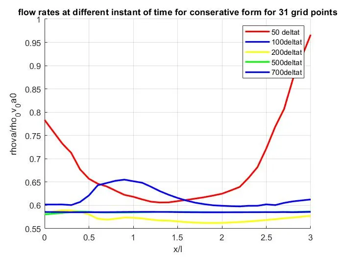
figure(7):flow rates at different instant of time for conservative for 31 grid points
from the above graph we can conclude that mass flow rate attains stablity after 700 time step for conservative form i,e the mass conserved after 700th time step.
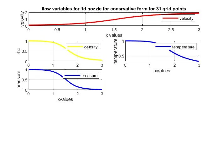
figure(8):flow variables for conseravative form for 31 grid points
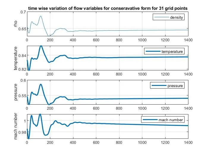
figure(9):flow variables variation for different time instant for conservative form for 31 grid points
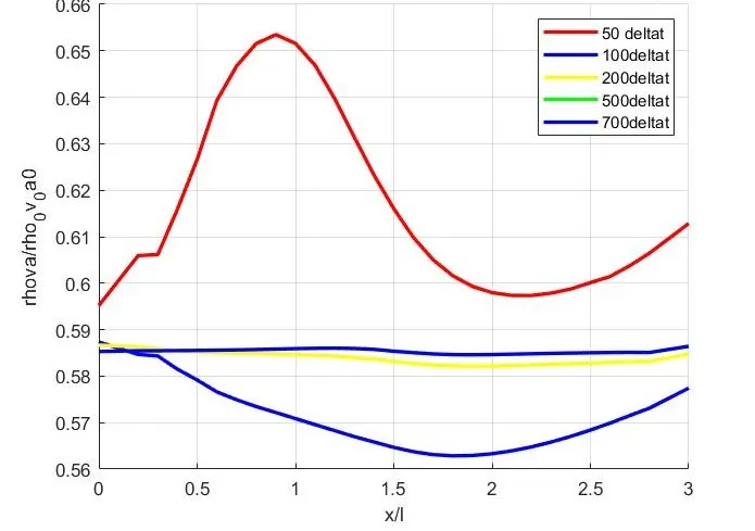
figure(10):flow rate at different instant of time for 61 grid points for conservative form
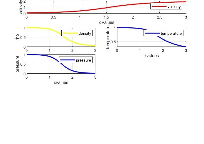
figure(11):flow variables for conservative form for 61 grid points
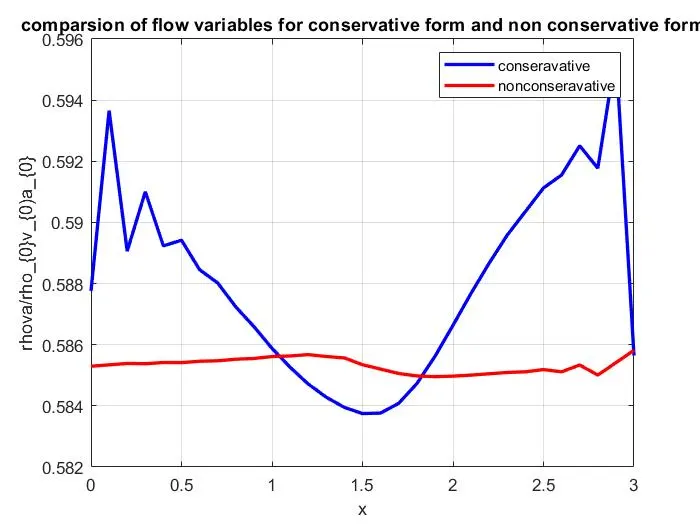
figure(12):comparision of flow rate bewteen conservative and non conservative for 31 grid points
from above graph we can say that the mass flow rate for conservative is almost similar to the analytical as mentioned in the book and time for simulation for non conservative is less than the conservative form.
| number of grid points | form of equation | rho/rho(throat) | t/t(throat) | pressure/pressure(throat) | mach number/mach number(throat) |
| 31 | nonconservative | 0.639 | 0.836 | 0.534 | 0.999 |
| 31 | conservative | 0.652 | 0.841 | 0.548 | 0.978 |
| 61 | non conservative | 0.638 | 0.835 | 0.532 | 1 |
| 61 | conservative | 0.639 | 0.835 | 0.528 | 1 |
from above tables the flow variables values are close to analytical even though we increase the number of grid points fror bpth conservative and non conservative form hence they are indepedent of grid points.
conclusion
1. the attaing of mass stablity is faster in non conservative than the conservative for hence the simulation of time is more for conservative than the non conservative form.
2.the mass flow rate is similar to the analytical in the coservative than in the non conservative form.
3.the flow variables are indepedent of number of grid points .