Week 7 - Simulation of a 1D Super-sonic nozzle flow simulation using Macormack Method
Nozzle - nozzle is used to control the velocity of fluid flow flowing through nozzle.
As area of the nozzle decreases, speed of fluid flow increases because when area decreases,
the pressure also decreases and the fluid flows fast due to decrease in pressure (Convergent type nozzle )
When area of the nozzle increases the fluid get more space to stay in the increased area,this causes increase in pressure at that area, therefore fluid flow velocity decreases when area increase(Divergent type nozzle)
In our case, the nozzle is convergent-divergent.(subsonic-supersonic)
In subsonic part, the mach number is less than 1(appropriately 0.65) and in supersonic part,the mach number is greater than 1 (appropriately 1.35)
In this project, our main objective is to perform the simulation of fluid flowing through convergent-divergent nozzle
For this,we are going to solve the quasi 1-Dimensional nozzle flow equation in matlab.
Conservative and non conservative forms of governing eqaution.
Governing pde's can be shown by different means
Conservative forms
Non-conservative form
Dimensional form
Non dimensional form
Conservative and non conservative forms are different in numerical discretization
Conservative and non conservative forms are meaningful when we solve them computationally,
Analytically they are menaning less.
The conservative form is more accurate than non conservative form.
It tends to work well with shocks or discontinuities exist in the domain.
About PDE.
Convert the integral form of governing equations into partial derivative form and also to follow quasi-one-dimensional assumption while doing this.
We will get pde's set of eqaution
(i.e continuity equation, momentum equation, energy equation)
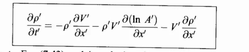
Continuity equation
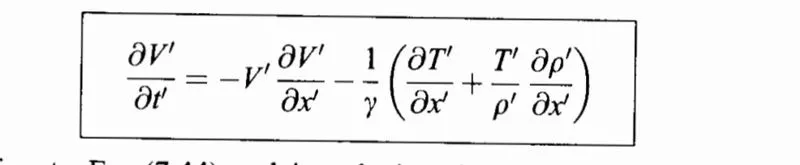
Momentum equation
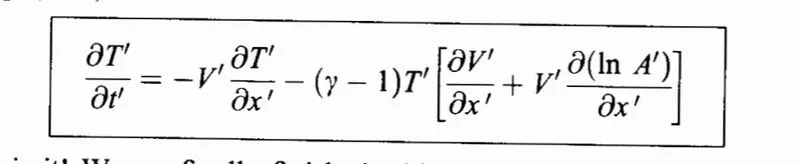
Energy equation in terms of temperature
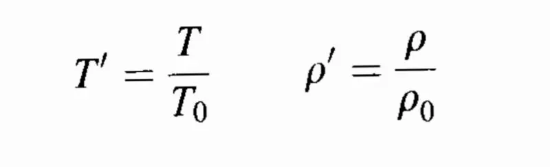
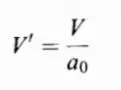
non dimensional temperature,density, area, time, velocity.
 ,
, 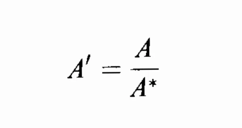 ,
, 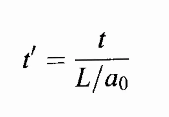 ,
, 
The above equations are the most convinient for time marching solution of quasi one dimensional flow and it is in non conservation and in dimensionless form.
Mostly the nozzle flow variables are expressed in non dimensional form
But to take dimensional form is also fine.
It depends completely on cfd engineer to which form to take for solving
There is no real difference as per the numerics are concerned.
Firstly, we are going to perform simulation by Non conservative form
The steps of the cfd are
Meshing
Descretization
Solving
In meshing
To mesh the 1-Dimensional domain of nozzle
(x direction) into number of grid points
In reality the flowfield variation in nozzle is in both x and y direction but we assumed that these variation is going to held in x direction only.
To solve the governing equations which are made appropriate for nozzle flow equations in matlab for each and every grid point of domain but excluding the boundary grid points because the initial and final values of variables are known there.
Discretization
The LHS of the governing equation has time derivatives
So the solution will be the time marching solutions
We are going to solve these equations explicitly.
Explicit scheme - The current solution for a variable is fully dependent on parameters at previous time.
MacCormack's technique
In this technique,we are going to split the time marching in two phase
Predicted step
corrector step
Predictor step
We start with the initial condition to calculate the value at next time step but it is not the complete time step, it is only the prediction step
Forward difference scheme is applied on RHS space terms
Solution update
In this step,with the help of predicted time derivative,the updated time marching term is been computed
Corrector step
In this step we find corrected value of time marching term.
Backward difference scheme is applied on space terms
Then the Average of predicted and corrected terms is calculated.
As we are solving this explicitly, the courant number stability criteria should get followed.
C should be less than 1.
Predictor step equation
(∂ρ/∂t)predicted = -ρiN[vNi+1 _ viN/Δx] – ρiN viN [ln(Ai+1) – ln(Ai)/Δx] – viN[ρi+1N – ρiN/Δx]
(∂v/∂t)predicted = -viN[vNi+1 _ viN/Δx] – (1/ϒ)[Ti+1N – TiN /Δx + Ti/ρiN(ρi+1N – ρiN/Δx)]
(∂v/∂t)predicted = -viN [Ti+1N – TiN /Δx] – (ϒ-1)TiN [vNi+1 _ viN/Δx + viN[ln(Ai+1) – ln(Ai)/Δx]
Updated solution
ρupdated = ρinitial condition + (∂ρ/∂t)predictedΔt
vupdated = vinitial condition + (∂v/∂t)predictedΔt
Tupdated = Tinitial condition + (∂v/∂t)predictedΔt
Corrector step
(∂ρ/∂t)corrector = -ρiN[vui _ vi-1u/Δx] - ρiu viu [ln(Ai) – ln(Ai-1)/Δx] – viu[ρiu – ρi-1u/Δx]
(∂v/∂t)corrector = -viu[vui _ vi-1u/Δx] – (1/ϒ)[Tiu – Ti-1u /Δx + Ti/ρiu(ρiu – ρi-1u/Δx)]
(∂T/∂t)corrector = -viu [Tiu – Ti-1u /Δx] – (ϒ-1)Tiu [vui _ vi-1u/Δx + viu[ln(Ai) – ln(Ai-1)/Δx]
Average of predicted and corrected
(∂ρ/∂t)average = 0.5 [ (∂ρ/∂t)predicted + (∂ρ/∂t)corrector ]
(∂v/∂t)average = 0.5 [ (∂v/∂t)predicted + (∂v/∂t)corrector ]
(∂T/∂t)average = 0.5 [ (∂T/∂t)predicted + (∂T/∂t)corrector ]
We considered steady, isentropic flow through convergent divergent nozzle
The flow at inlet to the nozzle comes from a reserviour where the pressure and temperature are denoted by Po and To respectively
The flow expands to supersonic speed at the exit of nozzle
At throat (M = 1)
We made assumption that the flow properties varies only with respect to x
Such flow is quasi one dimensional flow.
The flow field variables changes from one time step to next
As the time step proceeds ,the flow field variables approaches to zero(i.e the steady state gets achieved)
MATLAB CODING FOR NON-CONSERVATION
FUNCTION FOR PREDICTOR STEP
% function for predictor method

function [Continuity,Momentum,Energy] = non_conservation_pr(rho,v,t,a,j,dx,gamma)

drhodx = (rho(j+1)-rho(j))/dx;
dvdx = (v(j+1)-v(j))/dx;
dtdx = (t(j+1)-t(j))/dx;
dlog_adx = (log(a(j+1))-log(a(j)))/dx;

% continuity equation

Continuity = -rho(j)*dvdx - rho(j)*v(j)*dlog_adx - v(j)*drhodx;

% Momentum equation

Momentum = -v(j)*dvdx - (1/gamma)*(dtdx + (t(j)/rho(j))*drhodx);

% Energy equation in terms of temperature

Energy = -v(j)*dtdx - (gamma-1)*t(j)*(dvdx + v(j)*dlog_adx);

end
FUNCTION FOR CORRECTOR STEP
 function for corrector method

function [Continuity,Momentum,Energy] = non_conservation_cr(rho,v,t,a,j,dx,gamma)

drhodx = (rho(j)-rho(j-1))/dx;
dvdx = (v(j)-v(j-1))/dx;
dtdx = (t(j)-t(j-1))/dx;
dlog_adx = (log(a(j))-log(a(j-1)))/dx;

% continuity equation

Continuity = -rho(j)*dvdx - rho(j)*v(j)*dlog_adx - v(j)*drhodx;

% Momentum equation

Momentum = -v(j)*dvdx - (1/gamma)*(dtdx + (t(j)/rho(j))*drhodx);


% Energy equation in terms of temperature

Energy = -v(j)*dtdx - (gamma-1)*t(j)*(dvdx + v(j)*dlog_adx);

end
For both corrector and predictor, the name of a function should be the name of the file.
main code
% The program for macCormak technique

clear
close all
clc

% giving inputs

n = 31; % Number of grid points/Nodes
L = 3;
x = linspace(0,L,n);
dx = x(2)-x(1);
gamma = 1.4;

% Initial Conditions

rho = 1 - 0.3146*x;
t   = 1 - 0.2314*x;   % t = temperature
v   = (0.1 + 1.09*x).*t.^0.5;

% area
 a = 1+2.2*(x - 1.5).^2;

 % Time step

 nt = 800;

 % C = to assign the courant number which stabilizes the solution
 C = 0.5;
 dt = min((C.*dx)./(sqrt(t)+v));   % a = squareroot of t (t = temperature)

 % time loop
 tic;
 for k = 1:nt

     rho_old = rho;
     v_old = v;
     t_old = t;


     % predictor step

     for j = 2:n-1

     [drho_dt_pr(j),dvdt_pr(j),dtdt_pr(j)] = non_conservation_pr(rho,v,t,a,j,dx,gamma);


     % solution update step

     rho(j) = rho(j) + drho_dt_pr(j)*dt;
     v(j)   = v(j) + dvdt_pr(j)*dt;
     t(j)   = t(j) + dtdt_pr(j)*dt;

     end
    % Corrector step
    for j = 2:n-1

        [drho_dt_cr(j),dvdt_cr(j),dtdt_cr(j)] = non_conservation_cr(rho,v,t,a,j,dx,gamma);

    end

    % average of predicted and corrector terms

    drhodt = 0.5*(drho_dt_pr + drho_dt_cr);
    dvdt =   0.5*(dvdt_pr + dvdt_cr);
    dtdt =   0.5*(dtdt_pr +dtdt_cr);

    % final solution update

    for i = 2:n-1

        rho(i) = rho_old(i) + drhodt(i)*dt;
        v(i)   = v_old(i) + dvdt(i)*dt;
        t(i)   = t_old(i) + dtdt(i)*dt;

    end

    % boundary conditions


   % Inlet BC
   v(1) = 2*v(2) - v(3);

    % Outlet BC

    rho(n) = 2*rho(n-1)-rho(n-2);
    v(n) = 2*v(n-1) - v(n-2);
    t(n) = 2*t(n-1) - t(n-2);

    m = rho.*a.*v;      % mass flow rate
    mach = v./(sqrt(t));
    P = rho.*t;        % t = temperature

    % Solution Update at Throat

    rho_throat(k) = rho(16);
    temp_throat(k) = t(16);
    P_throat(k) = P(16);
    mach_th(k)  = mach(16);
    v_throat(k) = v(16);
    m_throat(k) = m(16);
    k_throat = 1:nt;

    toc


    % Variation of mass flow rate distribution inside the nozzle at
    % different time steps

      figure(1)
      hold on
      if k == 50
      plot(x,m);
      elseif k==200
      plot(x,m,'o')
      elseif k == 300
      plot(x,m);
      elseif k == 500
      plot(x,m,'r')
      grid on
      title('Mass flow rate at different time steps','Fontsize',15)
      xlabel('Non dimensional distance through nozzle','Fontsize',15)
      ylabel('non dimensional mass flow rate','Fontsize',15)
      end
 end


 % Steady state distribution of primitive variables inside the nozzle

 figure(2)
 subplot(2,3,1)
 plot(x,v,'Linewidth',2)
 title('velocity profile','Fontsize',15)
 xlabel ('x/L')
 ylabel('velocity ratio')
 grid on

 subplot(2,3,2)
 plot(x,rho,'Linewidth',2)
 title('density profile','Fontsize',15)
 xlabel('x/L')
 ylabel('density ratio')
 grid on

 subplot(2,3,3)
 plot(x,t,'Linewidth',2)
 title('   temp profile','Fontsize',15)
 xlabel('x/L')
 ylabel('temperature ratio')
 grid on

 subplot(2,3,4)
 plot(x,mach,'Linewidth',2)
 title('Mach number','Fontsize',15)
 xlabel('x/L')
 ylabel('Mach number')
 grid on

 subplot(2,3,5)
 plot(x,P,'Linewidth',2)
 title('pressure profile','Fontsize',15)
 xlabel('x/L')
 ylabel('Pressure ratio')
 grid on


 % time wise variation of primitive variations
  figure(3)
  subplot(2,2,1)
  plot(rho_throat,'Linewidth',2)
  title('density profile at throat','Fontsize',15)
  xlabel('time step')
  ylabel('density ratio')

  subplot(2,2,2)
  plot(temp_throat,'Linewidth',2)
  title('temp profile at throat','Fontsize',15)
  xlabel('time step')
  ylabel('temperature ratio')

  subplot(2,2,3)
  plot(P_throat,'Linewidth',2)
  title('pressure profile at throat','Fontsize',15)
  xlabel('time step')
  ylabel('pressure ratio')

  subplot(2,2,4)
  plot(m_throat,'Linewidth',2)
  title(' Mach no profile at throat','Fontsize',15)
  xlabel('time step')
  ylabel('M')


 % NORMALIZED MASS FLOW RATE

 figure(4)
 plot(x,m,'Linewidth',2)
 title('Normalized mass flow rate','Fontsize',15)
 xlabel('x/L')
 ylabel('mass flow rate')
 grid on
output
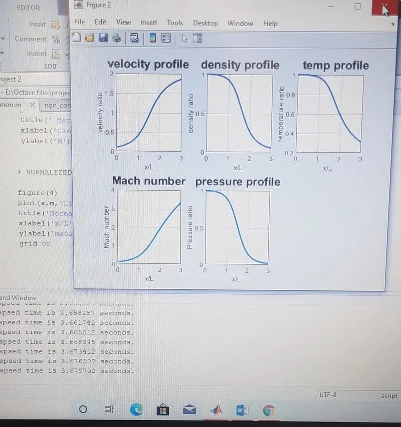
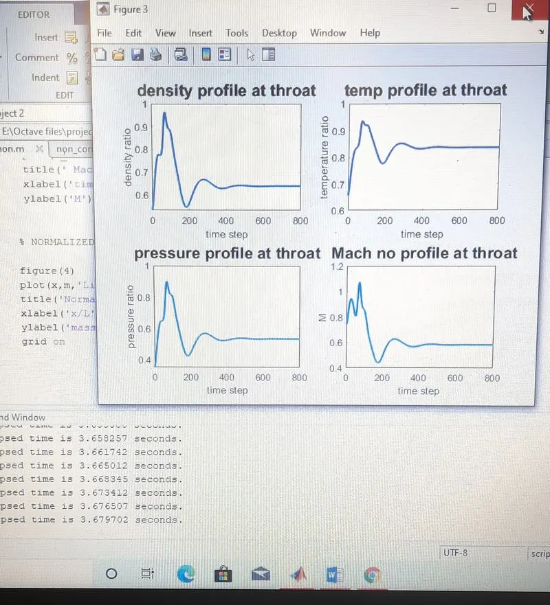
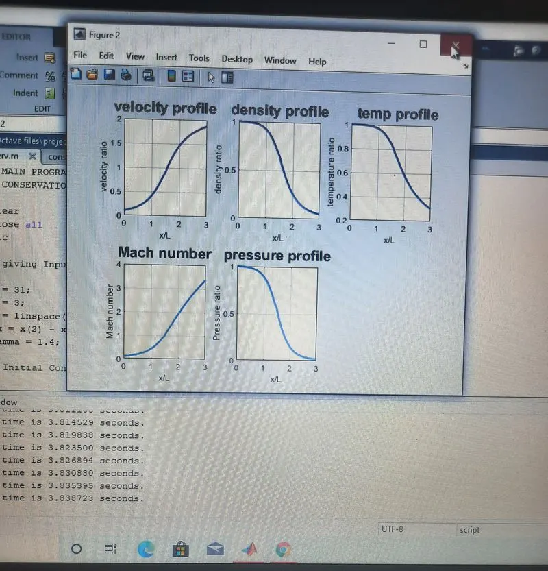
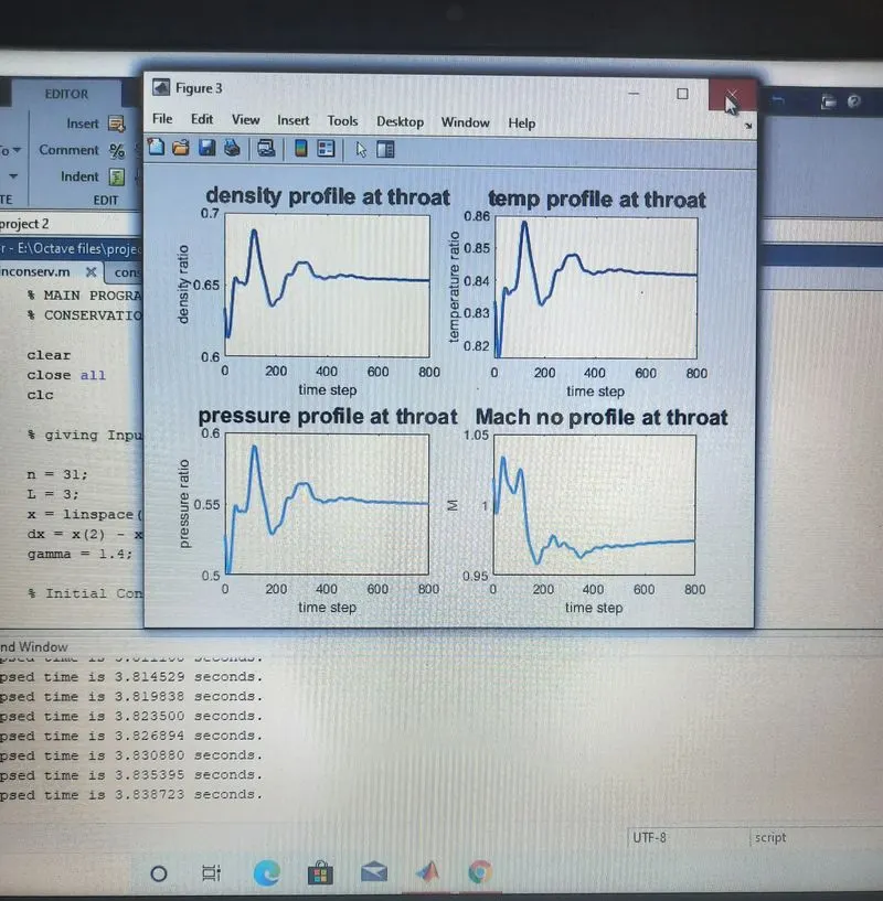
(Diagram 1) variation of primitive variables with nozzle length. (Diagram 2) variation of primitive variables with time step
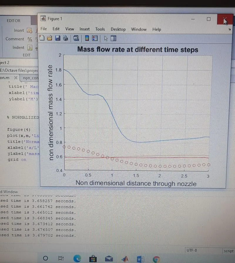
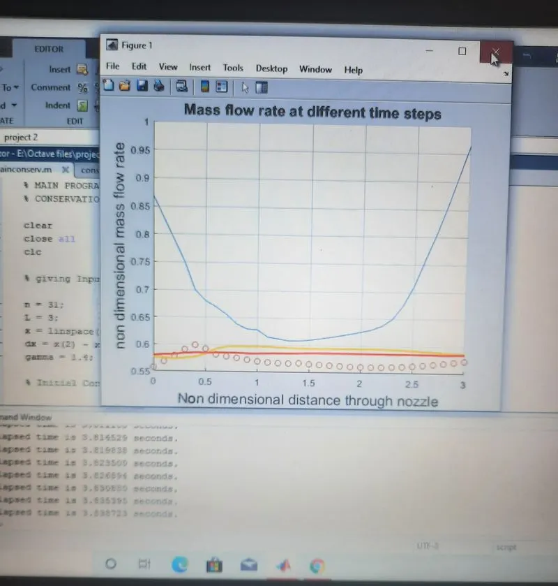
(Diagram 3) Mass flow rate at different time steps
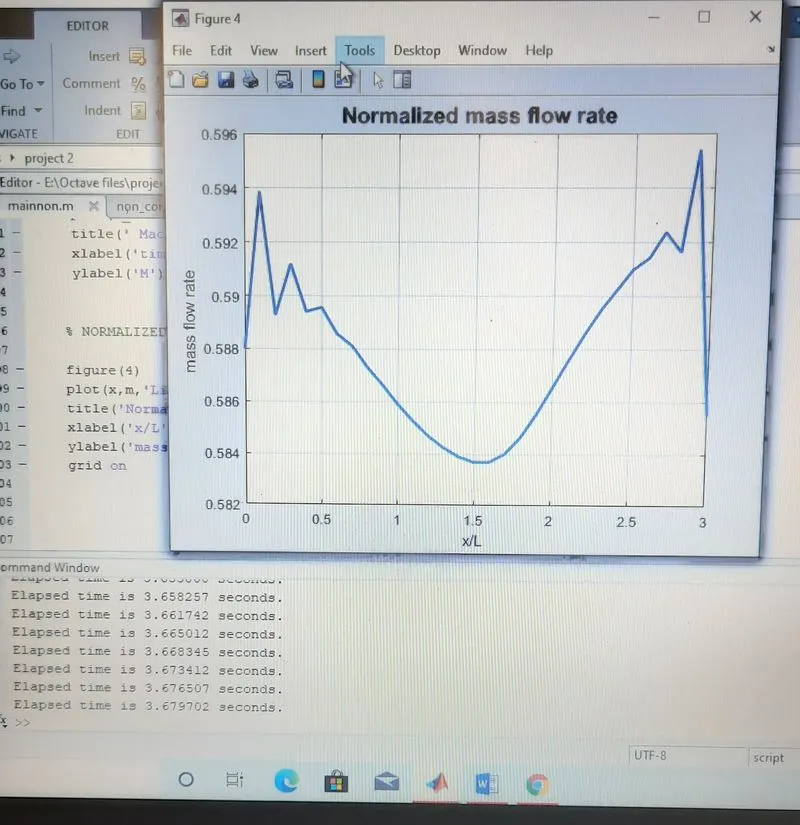
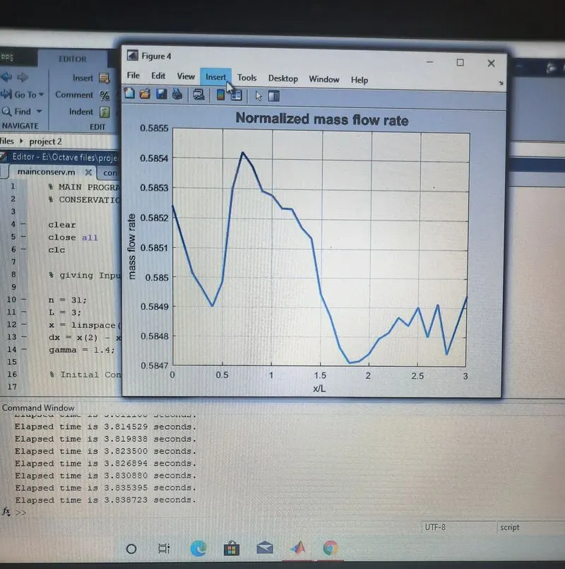
(Diagram 4) Normalized mass flow rate
simulation time for Non-Conservation form is 3.67 seconds for 31 grid points and at 800 time steps
CONSERVATION FORM
Continuity equation
∂(ρ’A’)/∂t’ + ∂(ρ’A’v’)/∂x’ = 0
Momentum equation
∂(ρ’A’v’)/∂t’ + ∂[(ρ’A’v’2) + (1/ϒ)p’A’]/∂x’ = (1/ϒ)p’(∂A’/∂x’)
Energy equation
∂[ρ’(e’/ϒ-1 + (ϒ/2)v’2)A’]/∂t’ + ∂[ρ’(e’/ϒ-1 + (ϒ/2)v’2)A’v’ +p’A’v’]/∂x’ = 0
MATLAB CODING FOR CONSERVATION FORM
FUNCTION FOR PREDICTOR STEP
% CONSERVATION FORM

% function for Predictor step

function [Continuity,Momentum,Energy] = conservation_pr(t,a,i,dx,gamma,f1,f2,f3,rho)

     dadx  = (a(i+1)-a(i))/dx;
     df1dx = (f1(i+1)-f1(i))/dx;
     df2dx = (f2(i+1)-f2(i))/dx;
     df3dx = (f3(i+1)-f3(i))/dx;


     j2 = (rho.*t.*dadx)./gamma;    %%% p = rho.*t

     % continuity Equation

      Continuity = -df1dx;

     % Momentum Equation

       Momentum = -df2dx + j2(i);

     % Energy Equation

       Energy = -df3dx;

end
FUNCTION FOR CORRECTOR STEP
% FUNCTION FOR CORRECTOR STEP
% CONSERVATION FORM


function [Continuity,Momentum,Energy]= conservation_cr(t,a,i,dx,gamma,f1,f2,f3,rho)

     dadx  = (a(i)-a(i-1))/dx;
     df1dx = (f1(i)-f1(i-1))/dx;
     df2dx = (f2(i)-f2(i-1))/dx;
     df3dx = (f3(i)-f3(i-1))/dx;


 j2 = (rho.*t.*dadx)./gamma;     %%% p = rho.*t

     % continuity Equation

      Continuity = -df1dx;

     % Momentum Equation

       Momentum = -df2dx + j2(i);

     % Energy Equation

       Energy = -df3dx;

end
MAIN CODE
% MAIN PROGRAM FOR CONSERVATION BY MACCORMACK'S TECHNIQUE
% CONSERVATION FORM

clear
close all
clc

% giving Inputs

n = 31;
L = 3;
x = linspace(0,L,n);
dx = x(2) - x(1);
gamma = 1.4;

% Initial Condition

% area
a = 1+2.2*(x - 1.5).^2;

% density and temperature initial condition

rho = zeros(1,n);
t = zeros(1,n);
for i = 1:n
    if (x(i)>=0 && x(i)<=0.5)
     rho(i) = 1;
     t(i) = 1;
    elseif (x(i)>=0.5 && x(i)<=1.5)
        rho(i) = 1-0.366*(x(i)-0.5);
        t(i) = 1-0.167*(x(i)-0.5);
    elseif (x(i)>=1.5 && x(i)<=3.5)
         rho(i) = 0.634-0.3879*(x(i)-1.5);
         t(i) = 0.833-0.3507*(x(i)-1.5);
    end
end

% Velocity Condition

v = 0.59./(rho.*a);

% initial Condition for Solution

e = t;
p = rho.*t;
u1 = rho.*a;
u2 = rho.*a.*v;
u3 = rho.*a.*((e/(gamma-1)) + ((gamma/2)*v.^2));


%time steps

nt = 800;
C = 0.5;     % courant number stablity criteria
dt = min((C.*dx)./(sqrt(t)+v));   % a = squareroot of t (t = temperature)


% time loop
tic;
for k = 1:nt


    u1_old = u1;
    u2_old = u2;
    u3_old = u3;

    %flux terms in pure form

    f1 = u2;
    term1 = (u3./u1) - ((gamma/2)*((u2./u1).^2));
    f2 = ((u2.^2)./u1)+(u1.*term1.*(gamma-1))./(gamma);
    term2 = (gamma*(gamma-1)*(u2.^3))./(2*u1.^2);
    f3 =((gamma*u2.*u3)./u1)-term2;

    % Predictor method

    for i = 2:n-1

    % GOVERNING PDES

    [du1_dt_pr(i),du2_dt_pr(i),du3_dt_pr(i)] = conservation_pr(t,a,i,dx,gamma,f1,f2,f3,rho);

    % SOLUTION UPDATE

    u1(i)= u1(i) + du1_dt_pr(i)*dt;
    u2(i)= u2(i) + du2_dt_pr(i)*dt;
    u3(i)= u3(i) + du3_dt_pr(i)*dt;

    end

rho = u1./a;
v = u2./u1;
t = (gamma-1)*((u3./u1)- ((gamma*v.^2)/2));


 % update flux term in pure form

    f1 = u2;
    term1 = (u3./u1) - ((gamma/2)*((u2./u1).^2));
    f2 = ((u2.^2)./u1)+(u1.*term1.*(gamma-1))./(gamma);
    term2 = (gamma*(gamma-1)*(u2.^3))./(2*u1.^2);
    f3 =((gamma*u2.*u3)./u1)-term2;


% Corrector method

for i = 2:n-1

 [du1_dt_cr(i),du2_dt_cr(i),du3_dt_cr(i)] = conservation_cr(t,a,i,dx,gamma,f1,f2,f3,rho);

end

%calculating the average value

du1_dt = 0.5*(du1_dt_pr + du1_dt_cr);
du2_dt = 0.5*(du2_dt_pr + du2_dt_cr);
du3_dt = 0.5*(du3_dt_pr + du3_dt_cr);

%SOLUTION UPDATE

    for j = 2:n-1

    u1(j)= u1_old(j) + du1_dt(j)*dt;
    u2(j)= u2_old(j) + du2_dt(j)*dt;
    u3(j)= u3_old(j) + du3_dt(j)*dt;
    end

   % apply boundary coditions

   % INLET BC
   u1(1) = rho(1)*a(1);
   u2(1) = 2*u2(2) - u2(3);
   v(1) = u2(1)/u1(1);
   u3(1) = u1(1)*((t(1)/(gamma-1))+((gamma/2)*v(1)^2));


   % outlet bc

   u1(n) =2*u1(n-1) - u1(n-2);
   u2(n) =2*u2(n-1) - u2(n-2);
   u3(n) =2*u3(n-1) - u3(n-2);

   % Obtaining primitive varibles
   rho = u1./a;
   v = u2./u1;
   t = (gamma-1)*((u3./u1)- ((gamma*v.^2)/2));
   p = rho.*t;
   mach = v./(sqrt(t));
   m = rho.*a.*v;

   % Solution Update at Throat

    rho_throat(k) = rho(16);
    temp_throat(k) = t(16);
    p_throat(k) = p(16);
    mach_th(k)  = mach(16);
    v_throat(k) = v(16);
    m_throat(k) = m(16);
    k_throat = 1:nt;

    toc


    % Variation of mass low rate distribution inside the nozzle at
    % different time steps

      figure(1)
      hold on
      if k == 50
      plot(x,m);
      elseif k==200
      plot(x,m,'o')
      elseif k == 300
      plot(x,m,'y','Linewidth',2)
      elseif k == 500
      plot(x,m,'r','Linewidth',2)
      grid on
      title('Mass flow rate at different time steps','Fontsize',15)
      xlabel('Non dimensional distance through nozzle','Fontsize',15)
      ylabel('non dimensional mass flow rate','Fontsize',15)
      end

end


% Steady state distribution of primitive variables inside the nozzle

 figure(2)
 subplot(2,3,1)
 plot(x,v,'Linewidth',2)
 title('velocity profile','Fontsize',15)
 xlabel ('x/L')
 ylabel('velocity ratio')
 grid on

 subplot(2,3,2)
 plot(x,rho,'Linewidth',2)
 title('density profile','Fontsize',15)
 xlabel('x/L')
 ylabel('density ratio')
 grid on

 subplot(2,3,3)
 plot(x,t,'Linewidth',2)
 title('   temp profile','Fontsize',15)
 xlabel('x/L')
 ylabel('temperature ratio')
 grid on

 subplot(2,3,4)
 plot(x,mach,'Linewidth',2)
 title('Mach number','Fontsize',15)
 xlabel('x/L')
 ylabel('Mach number')
 grid on

 subplot(2,3,5)
 plot(x,p,'Linewidth',2)
 title('pressure profile','Fontsize',15)
 xlabel('x/L')
 ylabel('Pressure ratio')
 grid on


  % Time wise variation of primitive variables

  figure(3)

  subplot(2,2,1)
  plot(rho_throat,'Linewidth',2)
  title('density profile at throat','Fontsize',15)
  xlabel('time step')
  ylabel('density ratio')

  subplot(2,2,2)
  plot(temp_throat,'Linewidth',2)
  title('temp profile at throat','Fontsize',15)
  xlabel('time step')
  ylabel('temperature ratio')

  subplot(2,2,3)
  plot(p_throat,'Linewidth',2)
  title('pressure profile at throat','Fontsize',15)
  xlabel('time step')
  ylabel('pressure ratio')

  subplot(2,2,4)
  plot(mach_th,'Linewidth',2)
  title('  Mach no profile at throat','Fontsize',15)
  xlabel('time step')
  ylabel('M')


 % NORMALIZED MASS FLOW RATE

 figure(4)
 plot(x,m,'Linewidth',2)
 title('Normalized mass flow rate','Fontsize',15)
 xlabel('x/L')
 ylabel('mass flow rate')
 grid on
OUTPUT
(diagram 1) variation of primitive variables with nozzle length. (diagram 2) variation of primitive variables with time step
(diagram 3) Mass flow rate at different time step
(Diagram 4) Normalized mass low rate.
For both conservative and non conservative form
The (diagram 1) are the distribution of primitive variables inside the nozzle for quasi 1D nozzle flow equation for 800 time step at 31 grid points
The variables changes as the nozzle length varies
(diagram 2)
the diagram 2 is the variation of primitive variables at throat where mach number is one
for both Non-conservative and conservative forms,at the initial time step there are much more variation but later as the time step increases the solution achieves steady state.
diagram (3)
mass flow rate at different time steps
for both Non-conservative and Conservative forms, we checked the mass flow rate at 50,200, 300,500 time steps and it shows that, as the time step proceeds, the solution achieves steadyness.
At 500 time step, it starts achieving steady state which is represented by red line in diagram 3
diagram(4)
Normalized mass flow rate
in non-conservation form,mass flow rate first increases then decreases at throat, then again increases in diverging section as per the convergent - divergent nozzle is concerned
In Conservation form, at nearer to throat, the mass flow rate is higher as compare to mass flow rate at throat in non conservation form,and it is true because as area decreases mass flow rate should increase
Simulation time
The simulation time for non conservation form is less than the simulation time for conservation form.This is because,the coding of non conservation form is not so complex as compare to conservaion form, also there are no flux terms present in it.
we conclude that for both forms, all the results are same excluding the results of mass flow rate distribution
grid point test
The velocity, mach number ,density, pressure, temperature does not have any major variation in graphs as number of nodes increases or we can say 'changes'.
but the mass flow rate have smooth changes because as number of nodes increases, we get the more information about mass flow rate in 3m length of nozzle.
non conservation form mass flow rate, at n = 61
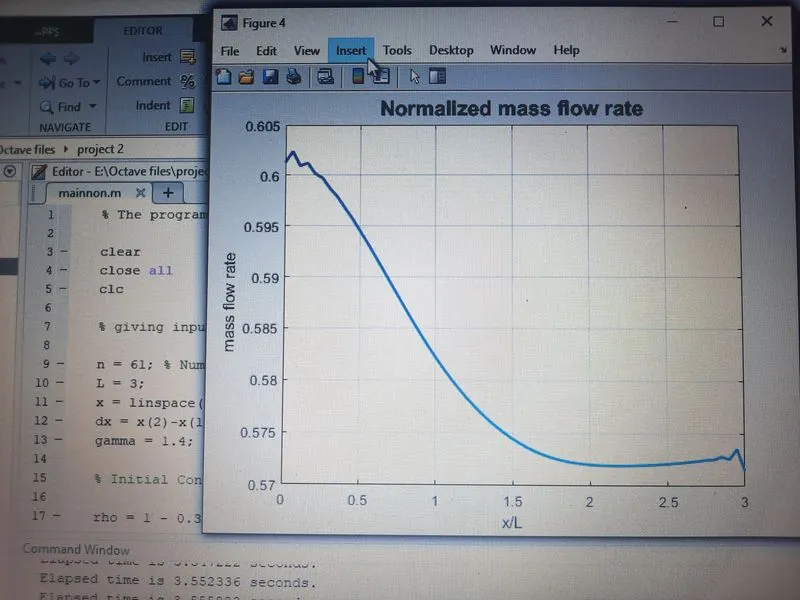
conservation form mass flow rate at n = 61
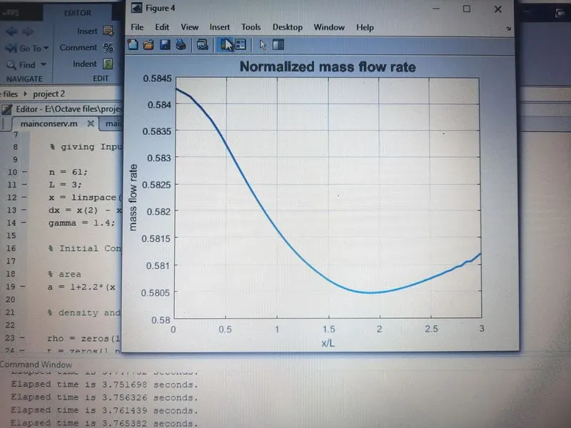
The mass flow rate graph is very much different at n = 31 and at n = 61
so appropriate number of nodes should be taken for the required mass flow rate and also the courant number stability criteria should get followed while choosing number of nodes
As number of grid points increases, simulation time also increases for both the cases