Week 5 - Mid term project - Solving the steady and unsteady 2D heat conduction problem
Our main objective is to perform the simulation of 2 dimensional heat conduction for a square domain
Boundary conditions
Top Boundary = 600 K
Bottom Boundary = 900 K
Left Boundary = 400 K
Right Boundary = 800 K
Steady state heat conduction - the heat flow rate from a solid or liquid does not change as the time proceeds or it remains constant or it is independent of time is called steady heat conduction.
Unsteady or transient heat conduction - heat conduction depends on time ( i.e) heat flow rate changes with time is called unsteady or transient heat conduction.
In this report, we are performing the heat conduction equation by two methods to get simulation nearer to the real solution
These methods are implicit and explicit.
As implicit methods equation is very complicated in solving,we use iterative solvers to solve the expanded form of equations
In this challenge, for implicit,we are using solvers which are
Jacobi
Gauss seidal
Successive over relaxation
Explicit method does not need solver,matlab itself solves the equation without solver because RHS side terms are known
But explicit schemes has lower accuracy which can cause bad optimization of simulation.
Due to this industries use implicit methods.
Let first simulate by EXPLICIT METHOD
In explicit method, the current solution for a parameter (in our case is Temperature) is fully dependent on parameters at previous time
The transient 2D heat conduction equation by explicit formula is given by
Tpn+1 = Tpn + k1(TR -2TP +TL)n +k2(TT -2Tp + TB)n
i.e the equation is
Tn+1i,j = Tni,j + k1(Ti-1,j – 2Ti,j + Ti+1,j)n +k2(Ti,j-1 -2Ti,j +Ti,j+1)n
k1 = alpha*dt/dx^2;
k2 = alpha*dt/dy^2;
Courant number stability terms.
Appropriate dt and nodes should be taken and CFL should be lower than 0.5 for a solution to be stable. this is because,this conduction equation is a time marching problem.
MATLAB CODE FOR TRANSIENT CONDUCTION BY EXPLICIT
close all
clc
clear


L = 1;
nx = 30;
ny = nx;
dt = 0.010;  % This is the time step between the two nodes
t  = 400;
nt = t/dt;
alpha = 0.0004;


x = linspace(0,L,nx);
dx = x(2)-x(1);
y = linspace(0,L,ny);
dy = y(2)-y(1);


%  temperatures of boundaries

T = 300*ones(ny,nx);  % initial condition
T(:,1) = 400;         % temperature at left boundary
T(:,end) = 800;       % temperature at right boundary
T(1,:) = 600;         % temperature at top boundary
T(end,:) = 900;       % temperature at bottom boundary
T_old = T;


k1 = alpha*dt/dx^2;   % courant number statement or formula
k2 = alpha*dt/dy^2;
CFL= k1+k2;

tic                   % tic command starts the time loop
iteration = 0;

% time loop
for k = 1:nt

% Y-space loop
    for j = 2:ny-1


% X-Space loop
for i = 2:nx-1
H = (T_old(i-1,j) - 2*T_old(i,j) + T_old(i+1,j));
V = (T_old(i,j-1) - 2*T_old(i,j) + T_old(i,j+1));
T(i,j) = T_old(i,j)+(H*k1)+(V*k2);
end
    end

T_old = T;
iteration = iteration +1
end
time = toc;     % toc command measures and express the simulation time


% plotting

[c,h] = contourf(x,y,T);
clabel(c,h)
colormap(jet)
ax = gca;
ax.YDir = 'reverse';     % This command reverse the y axis real numbers
xlabel('x')
ylabel('y')
pause(0.5)
title('TEMP profile by EXPLICIT method for transient conduction')
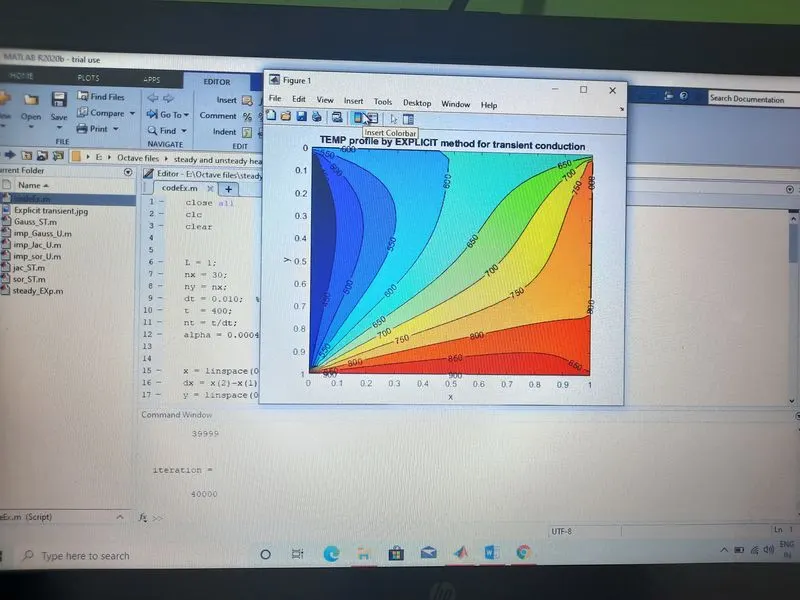
Updating the T_old = T is an important step because T_old is the initial temperature for next new T value which is going to cause the iterative loop.
contour is the command use to visualize simulation,
In EXPLICIT scheme, In our case, the dt is 0.010(assumed) which is very small and due this value, CFL numerical stability criteria gets followed and we achieved a steady state after the iterations
But if we increase the dt above 0.75, the solution diverges in a bad way, because CFL exceeds above 0.5 and this simulation becomes highly unstable
This tells us how CFL is crucial in explicit method.
It demands lower dt values
The corners temperature is not smooth if we are taking less or not taking appropriate number of nodes and it is true, because by taking less number of nodes we will have less information of temperature and due to this,it can cause small sudden changes in the temperature profile curves. this can affect economically in optimization of product.
TRANSIENT HEAT CONDUCTION BY IMPLICIT METHOD
In implicit method, the current solution of a parameter like Temperature is calculated with T at previous t and also T at current time.
The heat conduction equation in expanded form is by implicit formula is
Ti,jn+1 = Ti,jn + (alpha* dt) (Ti+1,j -2Ti,j + Ti-1,j/dx2)n+1 + alpha*dt (Tj+1,i – 2Ti,j + Tj-1,i/dy2)n+1
By rearranging, we can write the above equation as
Tpn+1 (1 +2k1 +2k2) = Tpn + k1(TL + TR)n+1 +k2(TT + TB)n+1
further it can be written as
Tpn+1 (1 +2k1 +2k2) = Tpn +k1(Ti-1,j +Ti+1,j)n+1 + k2(Ti,j+1 +Ti,j-1)n+1 ---- 1
Now this is the final expanded implicit version of the heat conduction equation.
rhs will change according to the solver
MATLAB CODE FOR TRANSIENT HEAT CONDUCTION BY JACOBI SOLVER.
clear
close all
clc
% solving this implicit equation by jacobi solver

%Given values
L = 1;
nx = 30;     % Appriopriately assumed
ny = nx;
dt = 0.20;   % Appropriatey assumed
t = 300;
nt = t/dt;
alpha = 0.0004;  % this thermal diffusivity is assumed according to temperature range and according to numerical stability

x = linspace(0,L,nx);
dx = x(2)-x(1)

y = linspace(0,L,ny);
dy = y(2)-y(1);


T = 300*ones(ny,nx);  % initial condition
T(:,1) = 400;         % temperature at left boundary
T(1,:) = 600;         % temperature at top boundary
T(:,end) = 800;       % temperature at right boundary
T(end,:) = 900;       % temperature at bottom boundary
T_old = T;
T_prev = T;

k1 = alpha*dt/dx^2;
k2 = alpha*dt/dy^2;
CFL =k1+k2;
tolerance = 1e-4;

%iteration method

tic
iteration = 0;
for k = 1:nt
    error = 2;
    while error > tolerance
        for j = 2:ny-1
            for i = 2:nx-1
                term1 = 1/(1+(2*k1)+(2*k2));
                term2 = k1*term1;
                term3 = k2*term1;

                H = (T_old(i-1,j) + T_old(i+1,j));
                V = (T_old(i,j-1) + T_old(i,j+1));
                T(i,j) = (T_prev(i,j)*term1)+(H*term2)+(V*term3);
            end
        end
        error = max(max(abs(T-T_old)));
        T_old = T;
        iteration = iteration+1
    end
    T_prev = T;
end
time = toc;

% plotting
[c,h] = contourf(x,y,T);
clabel(c,h)
colormap(jet)
ax = gca;
ax.YDir = 'reverse';
xlabel('x')
ylabel('y')
pause(0.5)
title('temp profile by JACOBI solver for transient conduction')
MATLAB CODE FOR TRANSIENT HEAT CONDUCTION BY GAUSS SEIDAL SOLVER.
clear
close all
clc

% Gauss seidal method
%Given values
L = 1;
nx = 30;          %appropriately assumed
ny = nx;
dt = 0.20;           %appropriately assumed
t = 300;
nt = t/dt;
alpha = 0.0004;    % assumed acoording to temperature range

x = linspace(0,L,nx);    %meshing command
dx = x(2)-x(1)           % space between the two nodes

y = linspace(0,L,ny);
dy = y(2)-y(1);


T = 300*ones(ny,nx);  % initial condition
T(:,1) = 400;         % temperature at left boundary
T(1,:) = 600;         % temperature at top boundary
T(:,end) = 800;       % temperature at right boundary
T(end,:) = 900;       % temperature at bottom boundary
T_old = T;
T_prev = T;

k1 = alpha*dt/dx^2;     % courant number statement
k2 = alpha*dt/dy^2;
CFL = k1+k2;
tolerance = 1e-4;

%iteration method

tic
iteration = 0;
for k = 1:nt
    error = 2;
    while error > tolerance
        for j = 2:ny-1
            for i = 2:nx-1
                term1 = 1/(1+(2*k1)+(2*k2));
                term2 = k1*term1;
                term3 = k2*term1;

                H = (T(i-1,j) + T_old(i+1,j));
                V = (T(i,j-1) + T_old(i,j+1));
                T(i,j) = (T_prev(i,j)*term1)+(H*term2)+(V*term3);
            end
        end
        error = max(max(abs(T-T_old)));
        T_old = T;
        iteration = iteration+1
    end
    T_prev = T;
end
time = toc;

  % plotting


[c,h] = contourf(x,y,T);
clabel(c,h)
colormap(jet)
ax = gca;
ax.YDir = 'reverse';
xlabel('x')
ylabel('y')
pause(0.5)
title('temp profile by GAUSS SEIDAL SOLVER for transient conduction')
MATLAB CODE FOR TRANSIENT HEAT CONDUCTION BY SUCCESIVE OVER RELAXATION SLOVER
clear
close all
clc

% successive over relaxation method
%Given values
L = 1;
nx = 30;       % assumed
ny = nx;
dt = 0.20;       % appropriately assumed
t = 300;          % assumed
nt = t/dt;
alpha = 0.0004;   % appropriately assumed for a given temperature range

x = linspace(0,L,nx);
dx = x(2)-x(1);

y = linspace(0,L,ny);
dy = y(2)-y(1);

T = 300*ones(ny,nx);  % initial condition
T(:,1) = 400;         % temperature at left boundary
T(1,:) = 600;         % temperature at top boundary
T(:,end) = 800;       % temperature at right boundary
T(end,:) = 900;       % temperature at bottom boundary
T_old = T;
T_prev = T;

k1 = alpha*dt/dx^2;
k2 = alpha*dt/dy^2;
CFL = k1+k2;
tolerance = 1e-4;

%iteration method
omega = 1.2;
tic
iteration = 0;
for k = 1:nt
    error = 2;
    while error > tolerance
        for j = 2:ny-1
            for i = 2:nx-1
                term1 = 1/(1+(2*k1)+(2*k2));
                term2 = k1*term1;
                term3 = k2*term1;

                H = (T_old(i-1,j) + T_old(i+1,j));
                V = (T_old(i,j-1) + T_old(i,j+1));

                T(i,j) = (T_prev(i,j)*term1)+(H*term2)+(V*term3);
                T(i,j) = T_old(i,j)*(1-omega)+ (omega)*T(i,j);

            end
        end

        error = max(max(abs(T-T_old)));
        T_old = T;
        iteration = iteration+1
    end
    T_prev = T;
end
time = toc;

  % plotting

[c,h] = contourf(x,y,T);
clabel(c,h)
colormap(jet)
ax = gca;
ax.YDir = 'reverse';      % this command is to reverse Y values
xlabel('x')
ylabel('y')
pause(0.5)
title('temp profile by SOR method for transient conduction')
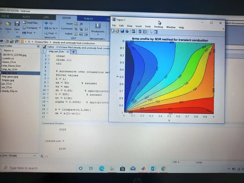
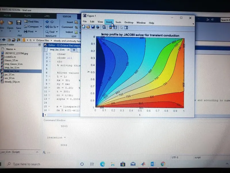
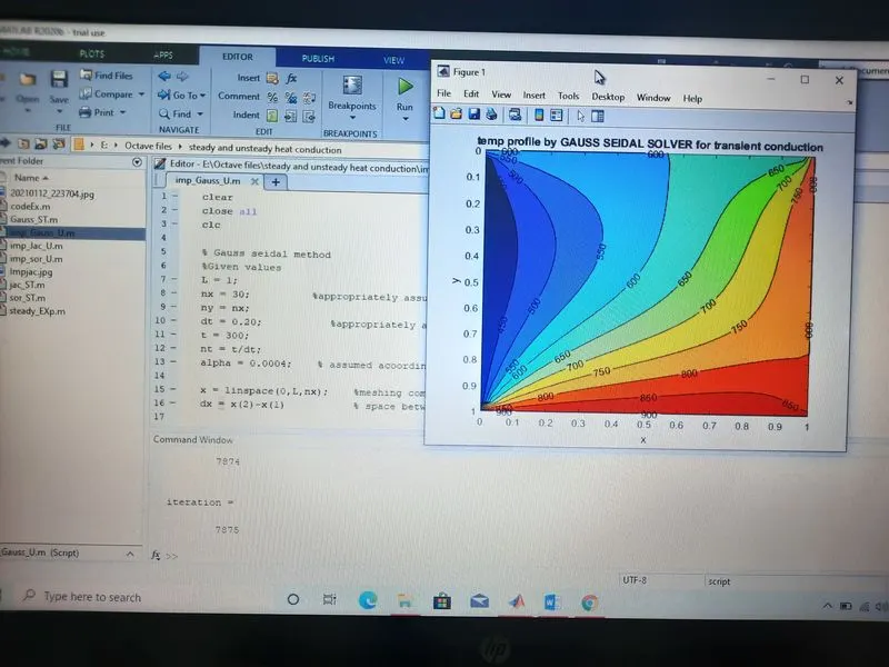
9843 JACOBI ITERATION > 7874 GAUSS SEIDAL ITERATION > 6338 SOR ITERATION
SIMULATION TIME FOR JACOBI > SIMULATION TIME FOR GAUSS SEIDAL > SIMULATION TIME FOR SOR ITERATION
here,SOR solver reaches the steady state with less number of iteration and less simulation time
also if the value of dt is increased i.e(high time steps),then there is no such a drastic change in the profile but simulation time varies. This clarifies that implicit schemes are stable
and we can input large dt to achieve steady state.
STEADY STATE ANALYSIS
The steady state heat conduction equation is
`del^2T/delx^2 +del^2T/dely^2 =0`
(TL – 2TP + TR / dx2) + (TT - 2TP + TB /dy2) = 0
By rearranging, we get
Tp*(2(dx2 + dy2)/dx2*dy2) = ((TL + TR) /dx2 + (TT +TB) /dy2)
k = (2(dx2 + dy2)/dx2*dy2
The final equation, we get
TP = (1/k)*((TL + TR) /dx2 + (TT +TB) /dy2)
Ti,j = (1/k)* ((Ti-1,j + Ti+1,j /dx2) +( Ti,j+1 + Ti,j-1/dy2 ) )
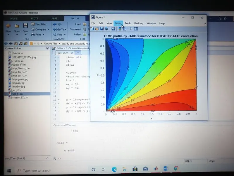
NOW TO SIMULATE STEADY HEAT CONDUCTION IMPLICITLY BY JACOBI SOLVER
close all
clc
clear

%Given
%Further using jacobi solver
L = 1;
nx = 30;
ny = nx;


x = linspace(0,L,nx);
dx = x(2)-x(1);
y = linspace(0,L,ny);
dy = y(2)-y(1);


%  temperatures of boundaries

T = 300*ones(ny,nx);  % initial condition
T(:,1) = 400;         % temperature at left boundary
T(:,end) = 800;       % temperature at right boundary
T(1,:) = 600;         % temperature at top boundary
T(end,:) = 900;       % temperature at bottom boundary
T_old = T;

Kterm = (dx^2*dy^2)/(2*(dx^2+dy^2));
tolerance = 1e-4;
error =1;
tic                   % tic command starts the time loop
iteration = 0;
while    error > tolerance

% Y-space loop
 for j = 2:ny-1


% X-Space loop
         for i = 2:nx-1
T(i,j)= Kterm*((T_old(i-1,j) + T_old(i+1,j))/(dx^2) +(T_old(i,j-1)+T_old(i,j+1))/(dy^2)); % jacobi form equation

         end
 end
error = max(max(abs(T-T_old)));
T_old = T;
iteration = iteration +1
end
time = toc     % toc command measures and express the simulation time


% plotting


[c,h] = contourf(x,y,T);
clabel(c,h)
colormap(jet)
ax = gca;
ax.YDir = 'reverse';
xlabel('x')
ylabel('y')
pause(0.5)
title('TEMP profile by JACOBI method for STEADY STATE conduction')
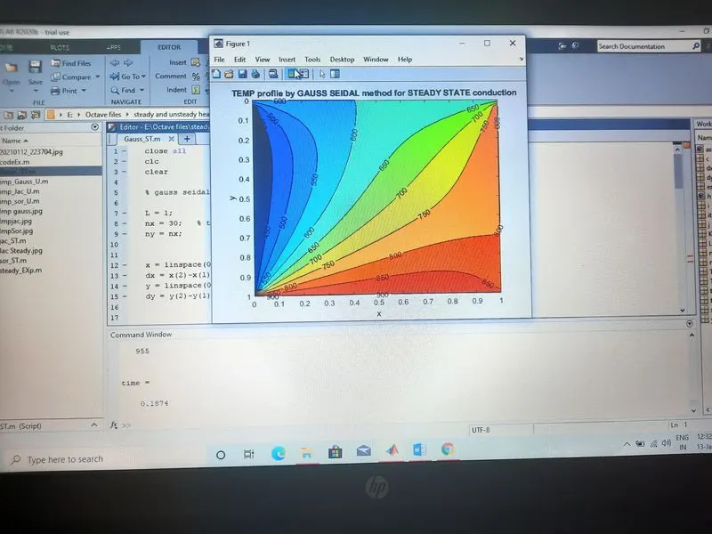
MATLAB CODE FOR STEADY STATE,SOLVING BY GAUSS SEIDAL SOLVER
close all
clc
clear

% gauss seidal

L = 1;
nx = 30;   % the one metre length will be get divided into 30 nodes
ny = nx;


x = linspace(0,L,nx);   %Meshing Command
dx = x(2)-x(1);
y = linspace(0,L,ny);
dy = y(2)-y(1);


%  temperatures of boundaries

T = 300*ones(ny,nx);  % initial condition
T(:,1) = 400;         % temperature at left boundary
T(:,end) = 800;       % temperature at right boundary
T(1,:) = 600;         % temperature at top boundary
T(end,:) = 900;       % temperature at bottom boundary
T_old = T;


% k1 = alpha*dt/dx^2   % courant number statement or formula
% k2 = alpha*dt/dy^2
% CFL= k1+k2

Kterm = (dx^2*dy^2)/(2*(dx^2+dy^2));
tolerance = 1e-4;
error =1;

tic                   % tic command starts the time loop
iteration = 0;
while  error > tolerance


% Y-space loop
        for j = 2:ny-1


% X-Space loop
   for i = 2:nx-1

 T(i,j)= Kterm*((T(i-1,j) + T_old(i+1,j))/(dx^2) +(T(i,j-1)+T_old(i,j+1))/(dy^2));

   end
        end

error = max(max(abs(T-T_old)));
T_old = T;
iteration = iteration +1

end
time = toc     % toc command measures and express the simulation time


% plotting


[c,h] = contourf(x,y,T);
clabel(c,h)
colormap(jet)
ax = gca;
ax.YDir = 'reverse';   % this commands reverse the Y AXIS
xlabel('x')
ylabel('y')
pause(0.5)
title('TEMP profile by GAUSS SEIDAL method for STEADY STATE conduction')
SOR SOLVER
close all
clc
clear

% SOR

L = 1;
nx = 30;
ny = nx;


x = linspace(0,L,nx);
dx = x(2)-x(1);
y = linspace(0,L,ny);
dy = y(2)-y(1);


%  temperatures of boundaries

T = 300*ones(ny,nx);  % initial condition
T(:,1) = 400;         % temperature at left boundary
T(:,end) = 800;       % temperature at right boundary
T(1,:) = 600;         % temperature at top boundary
T(end,:) = 900;       % temperature at bottom boundary
T_old = T;


% k1 = alpha*dt/dx^2   % courant number statement or formula
% k2 = alpha*dt/dy^2
% CFL= k1+k2

Kterm = (dx^2*dy^2)/(2*(dx^2+dy^2));
tolerance = 1e-4;
error =1;
omega = 1.2;
tic                   % tic command starts the time loop
iteration = 0;
while   error > tolerance
% time loop
% for k = 1:nt

% Y-space loop
  for j = 2:ny-1


% X-Space loop
      for i = 2:nx-1
T(i,j)= Kterm*((T(i-1,j) + T_old(i+1,j))/(dx^2) +(T(i,j-1)+T_old(i,j+1))/(dy^2));

T(i,j) = T_old(i,j)*(1-omega)+(omega)*T(i,j);
      end
  end
error = max(max(abs(T-T_old)));
T_old = T;
iteration = iteration +1
end
time = toc     % toc command measures and express the simulation time


% plotting


[c,h] = contourf(x,y,T);
clabel(c,h)
colormap(jet)
ax = gca;
ax.YDir = 'reverse';
xlabel('x')
ylabel('y')
pause(0.5)
title('TEMP profile by SOR method for steady state conduction')
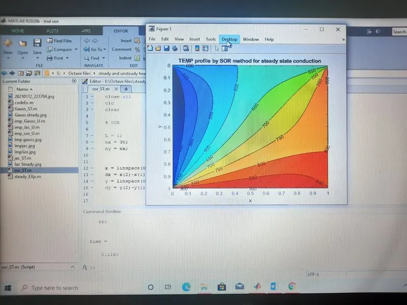
1783 JACOBI ITERATION > 955 GAUSS SEIDAL ITERATION > 660 SOR ITERATION
SIMULATION TIME FOR JACOBI > SIMULATION TIME FOR GAUSS SEIDAL > SIMULATION TIME FOR SOR ITERATION.
like in transient, we observe that,for steady state, simulation time and iteration is least in SOR method for given inputs.
hence in this report, for both steady and unsteady,we given the inputs and boundary conditions and done the meshing which comes in preprocessing
then we set the loop for solving the conduction equation , this comes in solving the equation(SOLVER)
and results (i.e contour plot) comes under postprocessing.