Week 9 - FVM Literature Review

The main objective is to explain the interpolation scheme and flux limiters in FVM.

We first go through the class of elliptic parabolic or hyperbolic equations, we choose Laplace equation,linear wave equation,transient heat conduction equation to solve the fluid flow problems and we get to known the importance of boundary conditions and decretization. But the actual fluid flow problems are very much complex. So we use General transport theorem for scalar property phi where we solve mixed advection-diffusion equation.

But as the flow becomes unsteady and turbulent and very much complex,we use the navier-stokes equation (i.e the group of continuity,momentum and energy equation.)
But to solve all above mentioned equations, a method is required.
There are three methods to solve the differential equations,particularly the partial differential equations .

These three methods are finite difference method, finite element method and finite volume method

We use finite difference method, finite element method or finite volume method as per the suitability of the problem.

With the help of these methods, we approximate the equations which becomes easy to solve?

FDM is used to discretise the physical domain into finite number of points.

FVM is used to discretise the physical domain into finite number of volumes.

In FDM, the derivative is replaced by an algebraic expression with the help of Taylor series.

In FVM, integral form of conservation equation are valid on finite control volume.

For FDM method to apply requires all the nodes linear or grid points aligned. Means it cannot be applied to unstructured mesh and non-orthogonal mesh.

In finite volume method, volume integrals in a pde form which contains a Divergence term are converted into surface integrals.
These terms are then evaluated as fluxes at the surfaces of each finite volume.
Because the flux entering is equal to flux leaving the adjacent volume.

steps of fvm methods

• Formal integration of the governing equations of fluid flow over all the control volumes of the solution domain
• Discretization involves the substitution of a variety of finite difference type approximations for the terms in the integrated equation representing flow processes such as convection,diffusion and sources.
• This converts integral equation into algebraic equations.
• Then further to solve algebraic by iterative method.

Types of finite volume grid

Cell centered approach

Cell centered approach is the most common approach in fvm in which the node is present at the centre of the control volume.

Face centered approach

Nodal locations are defined first and control volume are then constructed around them.

Both the approach are suitable for structured as well as for unstructured mesh.

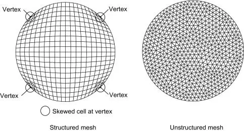
Interpolation schemes

• upwind interpolation scheme
• linear interpolation
• quadratic upwind interpolation
• hybrid interpolation scheme

Upwind interpolation scheme.

It is use for solving hyperbolic partial differential equations.

It senses the predominant direction of the flow and it consider it to interpolate the values at the face of the cell.

It only requires one cell in the upstream direction

It is first order accurate.

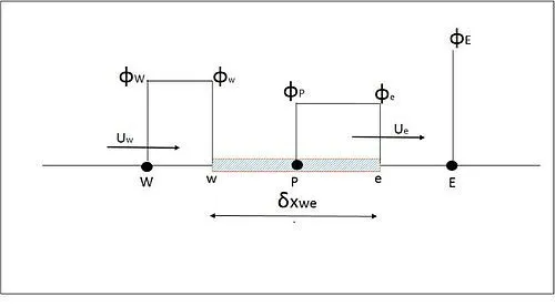
here the flow is from left to right .The value at east face (e) is equal to the value at upwind centroid P and the value at face w is equal to the value at upwind centroid W

ø_e = ø_P if mass flow rate at east face > 0

ø_e = ø_E if mass flow rate at east face < 0

ø_{w =} ø_P if mass flow rate at west face > 0

ø_w = ø_W if mass flow rate at west face < 0

Linear interpolation scheme

It is also called central difference scheme
because it is equivalent to the use of central difference formula of the first order derivative.

This scheme is used to approximate the value of variable at control volume face centre by two nearest computational node location.

It is second order accurate.

This scheme leads to simple approximation for evaluation of gradients required for evaluation of diffusive flux.

The solution can be oscillatory, hence we prefered small grids.

f_e = f_{E. `lambda`e} + f_p(1 –`lambda`­­_e)

_`lambda`e = (x_e – x_p)/(x_E – x_p)

QUICK(Quadratic upwind interpolation)

This scheme approximate the value of variable at control volume face centre by interpolation of three nearest nodes(one downstream and two uptream),
It is third order accurate for both uniform and non uniform grids

It stands for Quadratic Upstream Interpolation for Convective Kinematics

QUICK is most appropriate for steady flow or quasi-steady highly convective elliptic flow.

f_e = f_U +g₁(f_D – f_U) + g₂(f_UU – f_U)

g₁ = (x_e – x_U)(x_e – x_UU)/(x­_D –x_U).(x_D – x_UU)

g₂ = (x_e – x_U)(x_e –x_D)/(x_UU – x_U)(x_UU – x_D)

Hybrid interpolation scheme.

It is a combination of central difference and upwind scheme

f_e = ϒ.f_CDS + (1 – ϒ).f_UDS

FLUX LIMITERS

High resolution schemes are used in pde for higher accuracy, which is required in the presence of shocks vibrations or discontinuities in the problem.

Flux limiters are used in high resolution schemes to solve pde,particularly pde of fluid dynamics .

Flux limiter used in high-resolution scheme like MUSCL which stands for (monotonic Upstream centered scheme for conservation Laws) to avoid oscillations.

flux limiters are also called as slope limiters as they have same mathematical form and they can help in limiting the solution gradient near shocks and discontunities

Flux limiter + appropriate high-resolution schemes makes the solution TVD (total variation diminishing).

The main idea behind the construction of flux limiters is to limit the spatial derivatives into realistic values .


CHARM
HCUS
HQUICK
minmod are the common flux limiter

Consider 1D semi discrete scheme.

du_i//dt + (1/Δx_i)[F(u_i+1/2) – F(u_i-1/2)] = 0

where F(u_i+1/2) and F(u_i-1/2) represent edge fluxes for the ith cell.

If these edge fluxes can be represented by low and high resolution shemes, then a flux limiter can switch between these schemes depending upon the gradients close to the particular cell, as follows

F(u_i+1/2) = f^low_i+1/2 - ø(r_i)(f^low_i+1/2 - f^high_i+1/2)

F(u_i-1/2) = f^low_i-1/2 - ø(r_i-1)(f^low_i-1/2 - f^high_i-1/2)

Where f^low = low resolution flux.

f^high = high resolution flux.

Ø(r) = flux limiter function

r represents the ratio of successive gradients on the solution mesh

r_i = u_i –u_i-1/u_i+1-u_i