Week 7 - Simulation of a 1D Super-sonic nozzle flow simulation using Macormack Method
Convergent divergent nozzle or the supersonic nozzle or the delaval nozzle is used for supersonic flows. This has three sections: Subsonic section, throat, supersonic section.
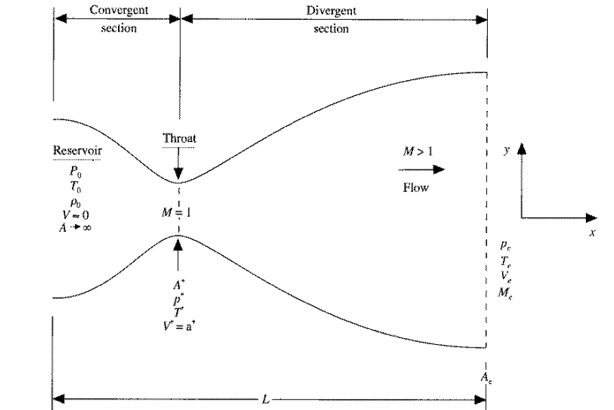
Fluid of low subsonic speed enter the subsonic section and the speed increases to the high subsonic speed at the end of the section. Fluid further increases the speed and reaches sonic speed at the throat. In the supersonic diverging section speed of the fluid becomes supersonic(Ma>1).
This nozzle is modelled using MacCormack's Method in both conservative and non-conservative forms of govering equations.
1.NON-CONSERVATIVE FORM:
Rho - Density
V- Velocity
T - Temperature
t - Time
A - Area
GOVERNING EQUATIONS:
Continuity Equation: `(delrho)/(delt)=-rho*(delV)/(delx) - rho*V*(delln(A))/(delx) - V*(delrho)/(delx)`
Momentum equation: `(delV)/(delt)=-V*(delV)/(delx) -(1/gamma)*(((delT)/(delx))+(T/rho)*((delrho)/(delx)))`
Energy equation : `(delT)/(delt)=-V*(delT)/(delx) - (gamma-1)*T[(delV)/(delx)+V(delln(A))/(delx)]`
BOUNDARY CONDITIONS AT t=0
`rho = 1-0.3146x`
`T = 1-0.2341x`
`V=(0.1+1.09x)T^(1/2)`
`a=(1 + 2.2(x-1.5)^2)`
INITIAL CONDITIONS
`V(n)=2V(n-1) - V(n-2)`
`rho(n)=2rho(n-1) - rho(n-2)`
`T(n)=2T(n-1) - T(n-2)`
`V(1)=2V(2)-V(3)`
`rho(1)=1`
`T(1)=1`
TIME STEP CALCULATION:
Most important factor of any simulation is stability of solution. It hightly depends on the value of time step increments. In this particular case time step can be calculated as:
`deltat=CFL*(deltax)/(a+V)`
where CFL is Courant Friedrichs Lowry (CFL) number which is determines the stability highly. Usually value of CFL must be less than 1 orelse solution will blow up as seen in previous challenges. Now, deltax is distance between each nodes, a is velocity of sound and V is local velocity. But velocity value will be changing at each and every point in this challenge so, minimum value from the above step is used as time step calculation of the solution. It's noted that for CFL above one solution isn't stable. As well CFL is 0.9 it takes lot of iteration than usal to converge. Hence 0.5 is idle CFL number for this challenge.
MACORMACK PROCEDURE:
For instance, assume we are calculating the continuity equation.
- First step in Macromack procedure is to find predictor value which uses forward marching for the taken equation. Which will be:
`(delrho)/(delt)=-rho*(V(i+1)-V(i))/(deltax) - rhoV*(lnA(i+1)-lnA(i))/(deltax) - V*(rho(i+1)-rho(i))/(deltax)`
similar procedure is done to the momentum and energy eqaution.
- Next step is to update all the three parameters given as boundary conditions for the next time step which can be done as:
`rho(t+deltat) = rho(t) + ((delrho)/(delt)(t)*deltat)` where density derivative is the one which obtained in previous step.
- Next step is corrector step which has to be done for the three governing eqauations. In this backward/rearward difference must be used. So corrector step for density dervivative can be calulated as:
`(delrho)/(delt)=-rho*(V(i)-V(i-1))/(deltax) - rhoV*(lnA(i)-lnA(i-1))/(deltax) - V*(rho(i)-rho(i-1))/(deltax)`and the similar procedure can be followed for velocity and temperature as well.
- Now the derivatives of the parameters obtained from corrector and predictor value should be averaged and then it should be updated in the next step. Density derivative can be done as:`((delrho)/(delt))avg = 0.5*[((delrho)/(delt))predic + ((delrho)/(delt))cor ]`where predictor and corrector derivative values are obtained from previous two stpes.
- `rho(t+deltat)=rho(t)+((delrho)/(delt))avg*deltat` this step will be repeated until it reaches a certain convergence.
- The same procedure can be used for conservative form as well just by replacing the governing equations and following the same steps.
Main Advantage of using MacroMack technique is that it will be using forward difference for predictor step and backward difference for corrector step. Both forward and backward difference methods are first-order approximation which just uses first-order differential equations. If we go for second-order central difference scheme it will be having second-order differential equations which take a lot of time for computation. Hence as an order of central difference goes up gradually time for solving too will take so long. So, it doesn’t mean the use of MacCormack technique (first-order) will yield poor result. Since it's taking corrector (backward method) and predictor(forward method) for computing and this average value is updated at each time step it will be accurate like second-order technique but it will take less amount of time than second order because of a lower-order partial differential equation.
CONSERVATIVE FORM:
Continuity Equation: `(del(rhoA))/(delt) = -(del(rhoAV))/(delx)`
Momentum Equation:`(del(rhoAV))/(delt) + (del(rhoAV^2+(1/gamma)rhoA))/(delx) = (1/gamma)p(delA)/(delx)`
Energy Equation: `(del[rho(e/(gamma-1)+gamma/2V^2)A])/(delt) + (del[rho(e/(gamma-1)+gamma/2V^2)VA+rhoAV])/(delx)=0` where e is internal energy
For ease of coding and debugging commom terms in above eqautions are taken out and inserted as follows:
`U1=rhoA`
`U2=rhoAV`
`U3=rho(e/(gamma-1)+gamma/2V^2)A`
`F1=rhoAV`
`F2=rhoAV^2`
`F3=rho(e/(gamma-1)+gamma/2V^2)VA+rhoAV`
`J2= (1/gamma)p(delA)/(delx)`
Thus the equations can be now can be written as:
Continuity equation:`(delU1)/(delt)=-(delF1)/(delx)`
Momentum Equation:`(delU2)/(delt)=-(delF2)/(delx)+J2`
Energy Equation :`(delU3)/(delt)=-(delF3)/(delx)`
BOUNDARY CONDITIONS:
for`0<=x<=0.5{rho=1 & T=1`
for `0.5<=x<=1.5{rho=1-0.366(x-0.5) & T=1-0.167(x-0.5)`
for `1.5<=x<=3{rho=0.634-0.3879(x-1.5) ; T=0.833-0.3507(x-1.5)`
MAIN PROGRAM:
close all
clear all
clc

%inputs
n=31;
x=linspace(0,3,n);
dx=x(2)-x(1);
gamma=1.4;
A = 1+ (2.2*(x-1.5).^2);
T=1-0.2134*x;
V=(0.1+1.09*x).*T.^0.5;
n_throat = find(A==1);
CFL=0.5;
dt = min(abs(CFL*dx./(realsqrt(T)+V)));
nt = 700;
%Non conservative form
tic
[rho,v,t,p,M,m,p_throat,rho_throat,v_throat,t_throat,M_throat]=nonconservative_2(n,x,dx,A,gamma,n_throat,nt,dt);
t1 = toc; %time

%conservative form
tic
[rho_ini,v_ini,T_ini,p_ini,M_ini,mdot,rho_throat_ini,v_throat_ini,T_throat_ini,M_throat_ini,p_throat_ini]=conservative_2(n,x,dx,A,gamma,n_throat,nt,dt);
t2 = toc; %time

%throat section
  figure(5);
  %non-conservative form
  %density ratio
  subplot(4,2,1);
  plot(rho_throat,'b');
  title('Change in density at throat with time in non-conservative form');
  ylabel('rho/rho_0');
  legend('density')
  xlabel('number of iteration');

  %Temperature
  subplot(4,2,3);
  plot(t_throat,'m');
  title('Change in temperature at throat with time in non-conservative form');
  ylabel('T/T_0');
  legend('Temperature')
  xlabel('number of iteration');

  %Pressure
  subplot(4,2,5);
  plot(p_throat,'g');
  title('Change in pressure at throat with time in non-conservative form');
  ylabel('P/P_0');
  legend('pressure')
  xlabel('number of iteration');

  %Mach number
  subplot(4,2,7);
  plot(M_throat,'r');
  title('Change in mach number at throat with time in non-conservative form');
  ylabel('M/M_0');
  legend('mach number')
  xlabel('Length');

%conservative form
% %Density ratio
 subplot(4,2,2);
 plot(rho_throat_ini,'b');
 title('Change in density at throat with time in conservative form');
 ylabel('rho/rho_0');
 legend('Density')
 xlabel('Length');

% %Temperature
 subplot(4,2,4);
 plot(T_throat_ini,'g');
 title('Change in temperature at throat with time in conservative form');
 ylabel('T/T0');
 legend('Temperature')
 xlabel('number of iteration');

 %Pressure
 subplot(4,2,6);
 plot(p_throat_ini,'m');
 title('Change in pressure at throat with time in conservative form');
 ylabel('P/P_0');
 legend('pressure')
 xlabel('number of iteration');

 %Mach number
 subplot(4,2,8);
 plot(M_throat_ini,'k');
 title('Change in mach number at throat with time in conservative form');
 ylabel('M/M_0')
 legend('mach number')
 xlabel('number of iteration');

 %comparison of mass flow
  figure(6)
  plot(x,m,'r')
  hold on
  plot(x,mdot,'b')
  xlabel('length')
  ylabel('mass-flow rate')
  text = sprintf('mass flow rate comparision');
  title(text)
  legend('nonconservative form','conservative form')
FUNCTION PROGRAM FOR NON-CONSERVATIVE FORM:
%non-conservative form of 1D supersonic nozzle flow equations

function [rho,v,t,p,M,m,p_throat,rho_throat,v_throat,t_throat,M_throat]=nonconservative_2(n,x,dx,A,gamma,n_throat,nt,dt)
%calculate initial profiles
rho=1-0.3146*x;
t=1-0.2134*x;  %t=temp
v=(0.1+1.09*x).*t.^0.5;
a=1+(2.2*(x-1.5).^2);

%outer time loop
for k=1:nt

    rho_old=rho;
    v_old=v;
    t_old=t;
    %predictor time step
    for j=2:n-1
        dvdx=(v(j+1)-v(j))/dx;
        drhodx=(rho(j+1)-rho(j))/dx;
        dTdx=(t(j+1)-t(j))/dx;
        dlogadx=(log(a(j+1))-log(a(j)))/dx;

        %continuity equation
        drhodt_p(j)=-rho(j)*dvdx -rho(j)*v(j)*dlogadx -v(j)*drhodx;
        %momentum equation
        dvdt_p(j)=-v(j)*dvdx-(1/gamma)*(dTdx + (t(j)/rho(j))*drhodx);
        %energy equation
        dTdt_p(j)= -v(j)*dTdx -(gamma-1)*t(j)*(dvdx+ ( v(j)*dlogadx));
        %solution update

        rho(j)= rho(j)+drhodt_p(j)*dt;
        v(j)= v(j)+ dvdt_p(j)*dt;
        t(j)= t(j)+ dTdt_p(j)*dt;
    end
    %Corrector method
     for j=2:n-1

        dvdx=(v(j)-v(j-1))/dx;
        drhodx=(rho(j)-rho(j-1))/dx;
        dTdx=(t(j)-t(j-1))/dx;
        dlogadx=(log(a(j))-log(a(j-1)))/dx;

        %continuity equation
        drhodt_c(j)=-rho(j)*dvdx -rho(j)*v(j)*dlogadx -v(j)*drhodx;
        %momentum equation
        dvdt_c(j)=-v(j)*dvdx-(1/gamma)*(dTdx + (t(j)/rho(j))*drhodx);
        %energy equation
        dTdt_c(j)= -v(j)*dTdx -(gamma-1)*t(j)*(dvdx+ ( v(j)*dlogadx));


    end
   %compute the average time derivative
   drhodt= 0.5*(drhodt_p + drhodt_c);
   dvdt= 0.5*(dvdt_p+dvdt_c);
   dTdt=0.5*(dTdt_p + dTdt_c);
   for i=2:n-1
       %final solution update
       rho(i)= rho_old(i) +drhodt(i) * dt;
       v(i)= v_old(i) +dvdt(i) * dt;
       t(i)= t_old(i) +dTdt(i) * dt;
   end

   %apply boundary condition
   %inlet
   rho(1)= 2*rho(2)- rho(3);
   v(1)= 2*v(2)- v(3);
   t(1)= 2*t(2)- t(3);
   %outlet
   rho(n)=2*rho(n-1)-rho(n-2);
   v(n)=2*v(n-1)-v(n-2);
   t(n)=2*t(n-1)-t(n-2);

   %Defining the non dimensional values of pressure and mass flow rate,Mach
   %number
   p=rho.*t;
   m = rho.*a.*v; %mass flow rate
   M = v./sqrt(t);
   %mdot=rho.*v.*A;

   %Parameters at the throat
   t_throat(k) = t(n_throat);
   p_throat(k) = p(n_throat);
   rho_throat(k) = rho(n_throat);
   v_throat(k) = v(n_throat);
   M_throat(k)= M(n_throat);

   %Throat section residual values
   rho_r(k) = drhodt(n_throat);
   t_r(k)= dTdt(n_throat);
   v_r(k)=dvdt(n_throat);

   %Comparision of mass flow rates at different times
   figure(1);
   hold on;
   if k ==1
     plot(x,m,'--')
   elseif k ==50
       plot(x,m,'r')
   elseif k ==100
           plot(x,m,'p');
   elseif k == 150
           plot(x,m,'b')
   elseif k==200
           plot(x,m,'g')
   elseif k==500
           plot(x,m,'*')
   elseif k==700
           plot(x,m,'v')
   end
end
  legend('deltat=0','deltat=50','deltat=100','deltat=150','deltat=200','deltat=500','deltat=700')
  legend('t=0','t=50','t=100','t=150','t=200');
  xlabel('x/L')
  ylabel('mass flow rate')
  title('Change in mass flow rate with time (non-conservative form')


  %Steady State Profiles
  figure(2);
  %Density Ratio
  subplot(4,1,1);
  plot(x,rho,'g');
  title('Steaty state profiles (non-conservative)');
  legend('Density Ratio');
  ylabel('rho/rho_0');

  %Temperature
  subplot(4,1,2);
  plot(x,t,'m');
  legend('Temperature');
  ylabel('T/T_0');

  %Pressure
  subplot(4,1,3);
  plot(x,p,'r');
  legend('Pressure');
  ylabel('p/p_0');

  %Mach number
  subplot(4,1,4);
  plot(x,M,'b');
  legend('Mach number');
  ylabel('M/M_0');
  xlabel('length');
end
FUNCTION PROGRAM FOR CONSERVATIVE FORM:
%Conservative form of 1D supersonic nozzle flow equations

function [rho_ini,v_ini,T_ini,p_ini,M_ini,mdot,rho_throat_ini,v_throat_ini,T_throat_ini,M_throat_ini,p_throat_ini]=conservative_2(n,x,dx,A,gamma,n_throat,nt,dt,CFL)

for i=1:length(x)
    if x(i)>=0 && x(i)<0.5
        rho_ini(i) = 1;
        T_ini(i) = 1;
    elseif x(i)>= 0.5 && x(i)< 1.5
        rho_ini(i) = 1- 0.366*(x(i)-0.5);
        T_ini(i)= 1- 0.167*(x(i)-0.5);
    elseif x(i)>= 1.5 && x(i) <=3
        rho_ini(i) = 0.634 - 0.3879*(x(i)-1.5);
        T_ini(i) = 0.833 - 0.3507*(x(i)-1.5);
    end
end

rho=rho_ini;
T=T_ini;
v_ini = (0.59)./(rho_ini.*A);
U=v_ini;


rho_old_ini = rho_ini;
v_old_ini = v_ini;
T_old_ini = T_ini;

% Initial conditions
U1 = rho_ini.*A;
U2 = rho_ini.*A.*v_ini;
U3 = rho_ini.*A.*((T_ini./(gamma-1))+((gamma/2)*(v_ini.^2)));

%Time loop
for j = 1:nt
    U1_old = U1;
    U2_old = U2;
    U3_old = U3;

    F1 = U2;
    F2 = ((U2.^2)./U1) + (((gamma-1)/gamma)*(U3 - ((gamma*0.5*(U2.^2))./U1)));
    F3 = ((gamma*U2.*U3)./U1) - ((gamma*0.5*(gamma-1)*(U2.^3))./(U1.^2));
    %Predictor step
    for k = 2:n-1
        dAdxj(k) = (1/gamma)*rho_ini(k)*T_ini(k)*((A(k+1)-A(k))/dx);

        %Continuity equation
        dU1dt_ini_p(k) = -(F1(k+1)-F1(k))/dx;

        %Momentum equation
        dU2dt_ini_p(k) = -((F2(k+1)-F2(k))/dx) + dAdxj(k);

        %Energy equation
        dU3dt_ini_p(k) = -(F3(k+1)-F3(k))/dx;

        %Predictor step update
        U1(k) = U1(k) + (dU1dt_ini_p(k)*dt);
        U2(k) = U2(k) + (dU2dt_ini_p(k)*dt);
        U3(k) = U3(k) + (dU3dt_ini_p(k)*dt);

    end


    %Predicted values
    rho_ini = U1./A;
    v_ini = U2./U1;
    T_ini = (gamma-1)*((U3./U1)-((gamma/2)*((U2./U1).^2)));
    p_ini = rho_ini.*T_ini;

    F1 = U2;
    F2 = ((U2.^2)./U1) + (((gamma-1)/gamma)*(U3 - ((gamma*0.5*(U2.^2))./U1)));
    F3 = ((gamma*U2.*U3)./U1) - ((gamma*0.5*(gamma-1)*(U2.^3))./(U1.^2));

    %corrector step
    for k = 2:n-1
        dAdxj(k) = (1/gamma)*rho_ini(k)*T_ini(k)*((A(k)-A(k-1))/dx);

        % Continuity Equation
        dU1dt_ini_c(k) = -(F1(k)-F1(k-1))/dx;

        %Momentum Equation
        dU2dt_ini_c(k) = -(F2(k)-F2(k-1))/dx + dAdxj(k);

        %Energy Equation
        dU3dt_ini_c(k) = -(F3(k)-F3(k-1))/dx;
    end

    %Average Time derivative

    dU1dt_ini_avg = 0.5*(dU1dt_ini_p + dU1dt_ini_c);
    dU2dt_ini_avg = 0.5*(dU2dt_ini_p + dU2dt_ini_c);
    dU3dt_ini_avg = 0.5*(dU3dt_ini_p + dU3dt_ini_c);

    %Final Solution Update
    for i = 2:n-1
        U1(i) = U1_old(i) + (dU1dt_ini_avg(i)*dt);
        U2(i) = U2_old(i) + (dU2dt_ini_avg(i)*dt);
        U3(i) = U3_old(i) + (dU3dt_ini_avg(i)*dt);
    end

    %Boundary Conditions
    %Inlet

    rho_ini = U1./A;
    v_ini = U2./U1;
    T_ini = (gamma-1)*(U3./U1-(gamma/2)*(v_ini.^2));

    U1(1) = rho_ini(1)*A(1);
    U2(1) = 2*U2(2)-U2(3);
    U3(1) = U1(1)*(T_ini(1)/(gamma-1)+(gamma/2)*(v_ini(1)^2));

    %Outlet
    U1(n) = 2*U1(n-1) - U1(n-2);
    U2(n) = 2*U2(n-1) - U2(n-2);
    U3(n) = 2*U3(n-1) - U3(n-2);

    %Calculation of properties

    p_ini = rho_ini.*T_ini;
    M_ini = v_ini./sqrt(T_ini);   %Mach number
    mdot = rho_ini.*A.*v_ini;

    %Properties at Throat
    rho_throat_ini(j) = rho_ini(n_throat);
    T_throat_ini(j) = T_ini(n_throat);
    M_throat_ini(j) = M_ini(n_throat);
    v_throat_ini(j) = v_ini(n_throat);
    p_throat_ini(j) = p_ini(n_throat);

    %Plotting change in mass-flow

     figure(3);
     hold on;

     if j==1
         plot(x,mdot,'*');
     elseif j==50
         plot(x,mdot,'--');
     elseif j==100
         plot(x,mdot,'b');
     elseif j==150
         plot(x,mdot,'r');
     elseif j==200
         plot(x,mdot,'g');
     elseif j==500
         plot(x,mdot,'y');
     elseif j==700
         plot(x,mdot);
     end

end
 title('change in Mass flow rate with time (Conservative Approach)')
 xlabel('x/L');
 ylabel('m/m_0');
 legend('t=0','t=50','t=100','t=150','t=200','t=500','t=700')
 axis([0 3 0 2]);

 %Steady state profiles of nozzle

 figure(4);
 %Density Ratio
 subplot(4,1,1);
 plot(x,rho_ini);
 title('Steady state profiles (conservative form)');
 legend('Density ratio');
 ylabel('rho/rho_0');

 %Temperature
 subplot(4,1,2);
 plot(x,T_ini);
 legend('Temperature');
 ylabel('T/T_0');

 %Pressure
 subplot(4,1,3);
 plot(x,p_ini);
 legend('Pressure');
 ylabel('p/p_0');

 %Mach number
 subplot(4,1,4);
 plot(x,M_ini);
 legend('Mach Number');
 ylabel('M/M0');
 xlabel('Length');

end
RESULTS:
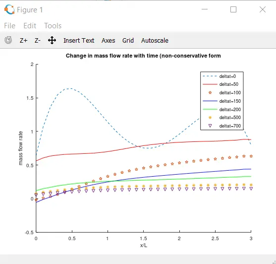
Mass flow rate comparison on different time steps in non-conservative method and conservative method.
In the below plots you can observe the non dimensional mass flow distribution across the nozzle at different time steps in both non conservative form and conservative form respectively.
1.non conservative method:
2. Conservative method:
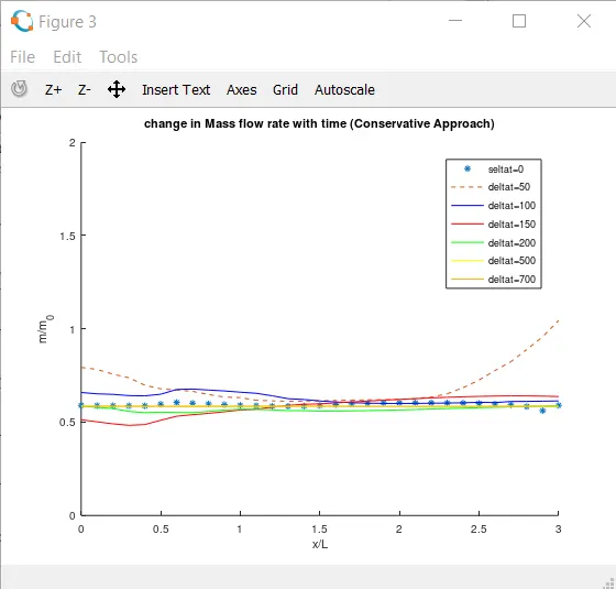
By observing the above plot you can conclude when the mass is conserved,in both the forms you can observe that it is conserved almost after 700 times steps.
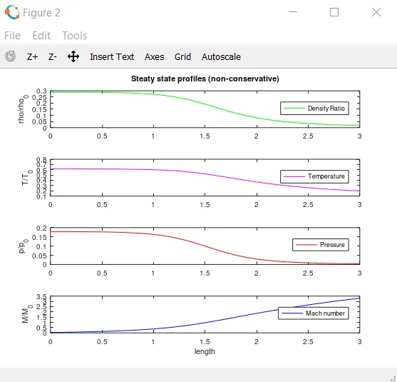
Steady state value of flow field variables:
1.Non-conservative form:
2.Conservative method:
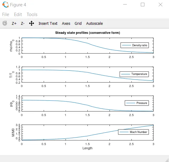
The above plots are almost same , when compared with the analytical solution from John D Anderson book.
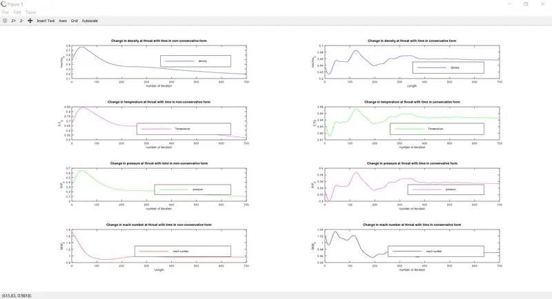
Timewise variation of flow field variable at throat in Non-conservative form&Conservative form
In the below plots you case see the timewise variation of non dimensional flow field variables at throat in both non conservative form and conservative form respectively attaining steady state.
normalized mass flow comparision between Non conservative method and conservative method: 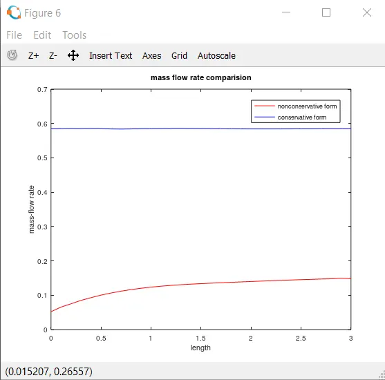
The comparison shown in above figure illustrates a general advantage of the conservation form of the equations. The conservation form does a better job of preserving mass throughout the flow field, mainly because the mass flow itself is one of the dependent variables in the equations,the mass flow is a primary result from these equations. In contrast, the dependent variables in the non conservation form of the equations are the primitive variables, and the mass flow is obtained only as a secondary result.
Conclusion:
1. The conservation form yields a better mass flow distribution. The conservation form simply does a better job of conserving mass since the mass flow itself is a dependent value.
2.There is no clear superiority of either form in terms of accuracy of the results. The nonconservation form seems to produce slightly more accurate results for the primitive variables, and the conservation form seems to produce slightly more accurate results for the flux variables. The results in either case are certainly satisfactory.
3 .Comparing the amount of calculational effort to achieve a solution, we note that the solution of the conservation form requires marginally more work. Most of this is due to the need to decode the primitive variables from the flux variables. such decoding is not necessary when you are solving the nonconservation form.
4.Non-conservative form attains steady state faster than the conservative form.
5.Both the forms conservative and non-conservative are grid independent.