Taylor table method and Matlab code

• We have set the grid points in our stencil along x plane.
• each grid points have its own taylor series functions.
• we have to create a taylor table from these sets of grid points

1.Fourth order approximation of second order derivative using Central difference method:

`Deltax^2(d^2f)/dx^2=a*f(i-2)+b*f(i-1)+c*f(i)+d*f(i+1)+e*f(i+2)`

Taylor's table

TERMS	f(i)	`Deltax**f'(i)`	`Deltax^2**f''(i)`	`Deltax^3**f'''(i)`	`Deltax^4**f^(iv)(i)`	`Deltax^5**f^(v)(i)`	`Deltax^6**f^(vi)(i)`
a*f(i-2)	a	-2a	4a/2	-8a/6	16a/24	-32a/120	64a/720
b*f(i-1)	b	-b	b/2	-b/6	b/24	-b/120	b/720
c*f(i)	c	0	0	0	0	0	0
d*f(i+1)	d	d	d/2	d/6	d/24	d/120	d/720
e*f(i+2)	e	2e	4e/2	8e/6	16e/24	32e/120	64e/720
`sum`	0	0	1	0	0

a+b+c+d+e=0-----------------(1)

-2a-b+d+2e=0-----------------(2)

2a+(b/2)+(d/2)+2e=1-------------(3)

-(4/3)a-(b/6)+(d/6)+(4/3)e=0------(4)

(2/3)a+(b/24)+(d/24)+(2/3)e=0---------(5)

converting equation 1,2,3,4&5 into matrix form

A=B*X

by solving above equation we get each terms ,

a=-1/12; b=4/3; c=-5/2; d=4/3; e=-1/12

and a=e&b=d

substituting above values in equation A and the equation A becomes

`(d^2f)/dx^2approx(a**f(i-2)+b**f(i-1)+c**f(i)+d**f(i+1)+e**f(i+2))/(Deltax^2)`

2. Fourth order approximation of second order derivative using skewed right sided difference method:

let,

`Deltax^2(d^2f)/dx^2approxa**f(i)+b**f(i+1)+c**f(i+2)+d**f(i+3)+e**f(i+4)+g**f(i+5)`----------(B`

Taylor's table

TERMS	f(i)	`Deltax**f'(i)`	`Deltax^2**f''(i)`	`Deltax^3**f'''(i)`	`Deltax^4**f^(iv)(i)`	`Deltax^5**f^(v)(i)`	`Deltax^6**f^(vi)(i)`
a*f(i)	a	0	0	0	0	0	0
b*f(i+1)	b	b	b/2	b/6	b/24	b/120	b/720
c*f(i+2)	c	2c	2c	4c/3	16c/24	32c/120	64c/720
d*f(i+3)	d	3d	9d/2	27d/6	81d/24	243d/120	729d/720
e*f(i+4)	e	4e	16e/2	64e/6	256e/24	1024e/120	4096e/720
g*f(i+5)	g	5g	25g/2	125g/6	625g/24	3125g/120	15625g/720
`sum`	0	0	1	0	0

a+b+c+d+e+g=0-----------(1)

b+2c+3d+4e+5g=0----------(2)

(b/2)+2c+(9d/2)+8e+(25g/2)=1------(3)

(b/6)+(4c/3)+(27d/6)+(64e/6)+(125g/6)=0------(4)

(b/24)+(16c/24)+(81d/24)+(256e/24)+(625g/24)=0-------(5)

converting above equation into matrix form

we get each values ,

a=15/4; b=-77/6; c=107/6; d=-13; e=61/12; g=-5/6

after substituting the values in equation B, then it becomes

`(d^2f)/dx^2approx(a**f(i)+b**f(i+1)+c**f(i+2)+d**f(i+3)+e**f(i+4)+g**f(i+5))/(Deltax^2)`

3.Fourth order approximation of second order derivative using skewed left sided difference method:

`(Deltax^2)(d^2f)/dx^2approxa**f(i)+b**f(i-1)+c**f(i-2)+d**f(i-3)+e**f(i-4)+g**f(i-5)`

Taylor's table

TERMS	f(i)	`Deltax**f'(i)`	`Deltax^2**f''(i)`	`Deltax^3**f'''(i)`	`Deltax^4**f^(iv)(i)`	`Deltax^5**f^(v)(i)`	`Deltax^6**f^(vi)(i)`
a*f(i)	a	0	0	0	0	0	0
b*f(i-1)	b	-b	b/2	-b/6	b/24	-b/120	b/720
c*f(i-2)	c	-2c	2c	-4c/3	16c/24	-32c/120	64c/720
d*f(i-3)	d	-3d	9d/2	-27d/6	81d/24	-243d/120	729d/720
e*f(i-4)	e	-4e	16e/2	-64e/6	256e/24	-1024e/120	4096e/720
g*f(i-5)	g	-5g	25g/2	-125g/6	625g/24	-3125g/120	15625g/720
`sum`	0	0	1	0	0

a+b+c+d+e+g=0-----------(1)

-b-2c-3d-4e-5g=0----------(2)

(b/2)+2c+(9d/2)+8e+(25g/2)=1------(3)

-(b/6)-(4c/3)-(27d/6)-(64e/6)-(125g/6)=0------(4)

(b/24)+(16c/24)+(81d/24)+(256e/24)+(625g/24)=0-------(5)

converting above equations into matrix form

after solving we get values of

a=15/4; b=-77/6; c=107/6; d=-13; e=61/12; g=-5/6

`(d^2f)/dx^2approx(a**f(i)+b**f(i-1)+c**f(i-2)+d**f(i-3)+e**f(i-4)+g**f(i-5))/(Deltax^2)`

Function program for central difference method:

function out=central_diff_approximation(x,dx)
  %f(x)=exp(x)*cos(x)
  %analytical derivative=f'(x)=exp(x)(cos(x)-sin(x))
  %f"(x)=-2*exp(x)*sin(x)
  analytical_derivative=-2*exp(x)*sin(x);
  
  %numerical derivative
  a=-1/12; b=4/3; c=-5/2; d=4/3; e=-1/12;
  
  %central differencing=(a*f(i-2)+b*f(i-1)+c*f(i)+d*f(i+1)+e*f(i+2))/(dx^2)
  central_differencing=((a*exp(x-(2*dx))*cos(x-(2*dx)))+(b*exp(x-dx)*cos(x-dx))+(c*exp(x)*cos(x))+(d*exp(x+dx)*cos(x+dx))+(e*exp(x+(2*dx))*cos(x+2*dx)))/(dx^2);
  out=abs(central_differencing-analytical_derivative)
endfunction

Function program for skewed right sided difference method:

function out=skewed_rigth(x,dx)
   %f(x)=exp(x)*cos(x)
  %analytical derivative=f'(x)=exp(x)(cos(x)-sin(x))
  %f"(x)=-2*exp(x)*sin(x)
  analytical_derivative=-2*exp(x)*sin(x);
  
  %numerical derivative
  a=15/4; b=-77/6; c=107/6; d=-13; e=61/12; g=-5/6;
  
  %skewed_rigth_sided_differencing=(a*f(i)+b*f(i+1)+c*f(i+2)+d*f(i+3)+e*f(i+4)+g*f(i+5))/(dx^2)
  skewed_rigth_sided_differencing=((a*exp(x)*cos(x))+(b*exp(x+dx)*cos(x+dx))+(c*exp(x+(2*dx))*cos(x+(2*dx)))+(d*exp(x+(3*dx))*cos(x+(3*dx)))+(e*exp(x+(4*dx))*cos(x+(4*dx)))+(g*exp(x+(5*dx))*cos(x+(5*dx))))/(dx^2);
  out=abs(skewed_rigth_sided_differencing-analytical_derivative)
endfunction

Function program for skewed left sided difference method:

function out=skewed_left(x,dx)
   %f(x)=exp(x)*cos(x)
  %analytical derivative=f'(x)=exp(x)(cos(x)-sin(x))
  %f"(x)=-2*exp(x)*sin(x)
  analytical_derivative=-2*exp(x)*sin(x);
  
  %numerical derivative
 a=15/4; b=-77/6; c=107/6; d=-13; e=61/12; g=-5/6;
  
  %skewed_rigth_sided_differencing=(a*f(i)+b*f(i-1)+c*f(i-2)+d*f(i-3)+e*f(i-4)+g*f(i-5))/(dx^2)
  skewed_left_sided_differencing=((a*exp(x)*cos(x))+(b*exp(x-dx)*cos(x-dx))+(c*exp(x-(2*dx))*cos(x-(2*dx)))+(d*exp(x-(3*dx))*cos(x-(3*dx)))+(e*exp(x-(4*dx))*cos(x-(4*dx)))+(g*exp(x-(5*dx))*cos(x-(5*dx))))/(dx^2);
  out=abs(skewed_left_sided_differencing-analytical_derivative)
endfunction

Main program:

clear all
close all
clc

x=pi/40;
dx=linspace(pi/4000,pi/40,20);

for i=1:length(dx)
  central_diff_approximation_error(i)=central_diff_approximation(x,dx(i));
  skewed_rigth_sided_error(i)=skewed_rigth(x,dx(i));
  skewed_left_sidede_error(i)=skewed_left(x,dx(i));
endfor
%ploting results
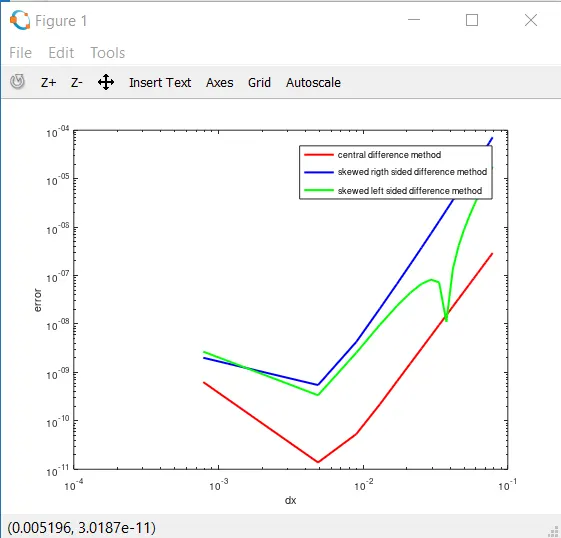
loglog(dx,central_diff_approximation_error,'linewidth',2,'r')
hold on
loglog(dx,skewed_rigth_sided_error,'linewidth',2,'b')
loglog(dx,skewed_left_sidede_error,'linewidth',2,'g')
xlabel('dx')
ylabel('error')
hold off
legend('central difference method','skewed rigth sided difference method','skewed left sided difference method')

Results:

Conclusion:

• From the figure we can observe central difference method has very less error. when we compare it with skewed method.
• errors of skewed right sided and skewed left sided are both look similar with the small difference in values.
• Here is the reason why skewed methods are usefull: When the system doesn't have both rigth and left nodes at the same time ,so we use skewed method.
• and CD method can't be used when the left and right node are not available at the same time. in this case we can use the skewed method.