Week 7: Shock tube simulation project

Objective:

• Setup a transient Shock tube simulation.
• Plot the pressure and temperature plots in the domain.
• Plot the cell count as a function of time.

Introduction:

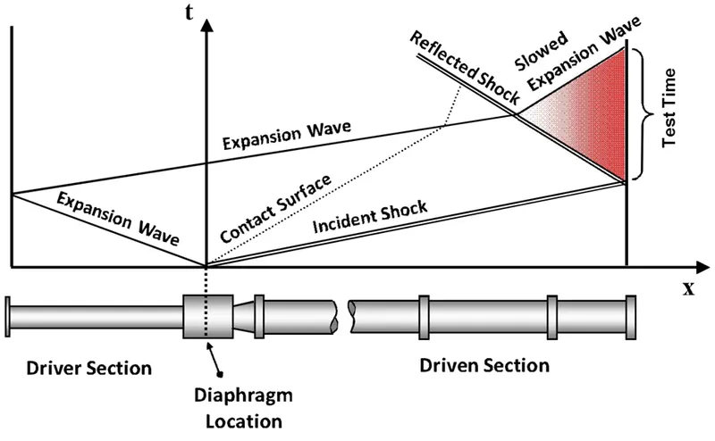
Shock tubes are ideal devices for studying combustion and chemical kinetics at high temperature and pressure. These devices produce these conditions by generating a shock wave to compress and heat the test gas (e.g. methane-air, etc.). A shock tube generates a shock wave using a section of high-pressure gas (referred to as driver section, usually filled with helium) and a section of low-pressure gas (driven section) separated by a diaphragm. Once the diaphragm ruptures, the driver and driven gases come into contact, creating a contact surface that acts as a piston compressing the test gas in the driven section and initiating shock wave propagation. The shock wave travels through the test gas in the driven section, then reflects from the closed endwall of the shock tube, causing further heating and compression of the test gas and stagnating it.

example for typical shock tube:

Geometry:

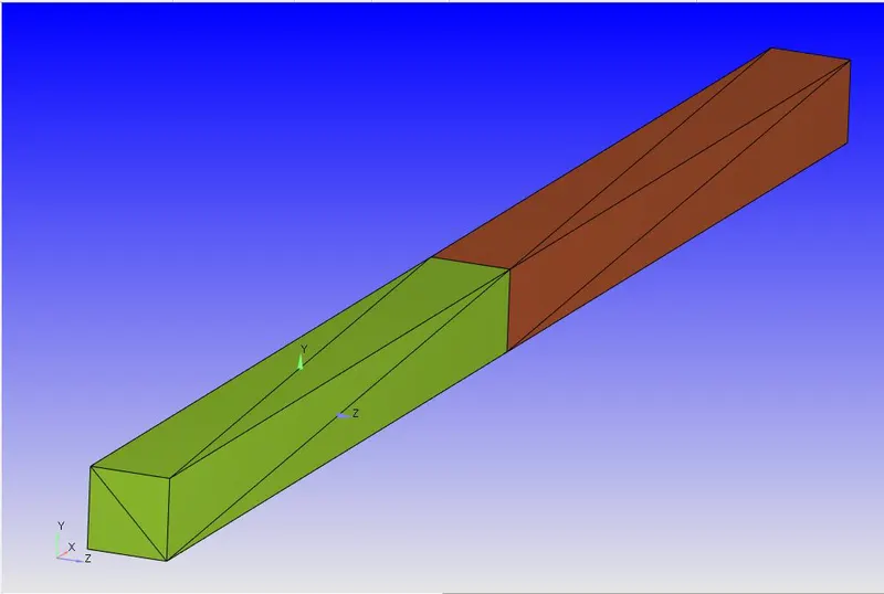
The green region is the High-pressure region and the brown one is the low-pressure region.

Dimensions of the shock tube:

Mesh Size:

It is a 2-dimensional simulation, hence along the z-direction, there is only one cell.

• in X-direction- 0.001 m
• in Y-direction- 0.001 m
• in Z-direction- 0.01 m

The Adaptive Mesh Refinement option is enabled. It refines the mesh of a selective region.For this simulation, the AMR is enabled for species criteria. The properties of AMR are kept as follows

• Maximum cells = 200000
• Maximum embedding level = 3
• Sub-grid criteria = 0.001

Mesh at t=0 sec

1. 
2. 

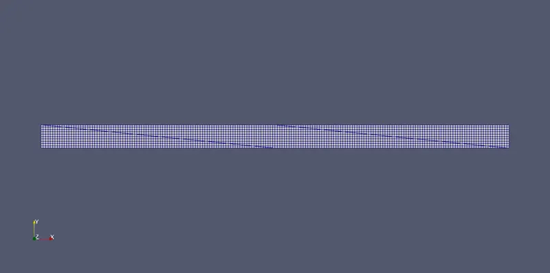
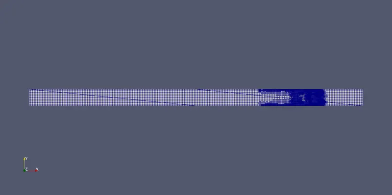
The effect of Adaptive Mesh Refinement can be observed in the video where the meshdevelops as the simulation progresses

Total cell counts:

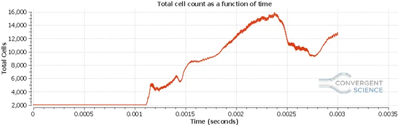
The maximum cell count is about 16000. Initially, it has a constant value of 2000 until thediaphragm breaks. The high-pressure N2 gas mixes with O2 and the mesh refinement begins as sub-grid criteria exceed the given value of 0.001.

Boundary Conditions:

The boundaries are grouped into two regions

• High pressure region
• Low pressure region

The set of boundary conditions in both these regions are identical.

• As the case is 2-dimensional, the front and the back wall of the tube are kept TWO_D.
• The sidewall has a boundary type WALL with No-slip boundary condition. The Temperatureand Turbulent Kinetic Energy have Dirichlet boundary condition at this wall.
• The Upper and Lower walls have a boundary type WALL with Law of Wall boundarycondition. The Temperature and Turbulent Kinetic Energy have Dirichlet boundary conditionat this wall.

Initial Conditions:

For the High-pressure region

For the Low-pressure region

• Pressure = 1.013 Mpa
• Temperature = 300 K
• Mass fraction of N2 = 0
• Mass fraction of O2 = 1

The Events option was enabled for this simulation. Using this option, we can simulate the function of a diaphragm as a physical diaphragm could not be accommodated in the geometry.

• The Diaphragm remains closed till 0.001 sec.
• After 0.001 sec, the diaphragm is opened and the gases start to mix in the domain.

RESULTS:

For Pressure

The pressure in High and Low-pressure zones (Region 0: High-pressure, Region 1: Low-pressure)

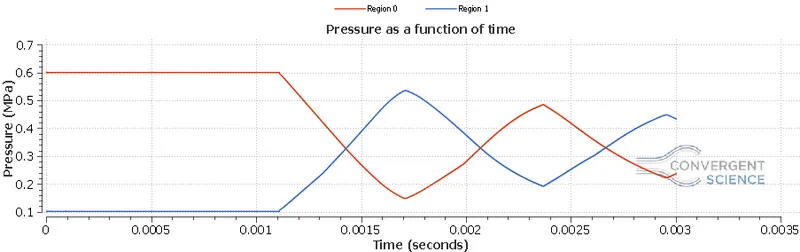
Pressure across the shock tube:

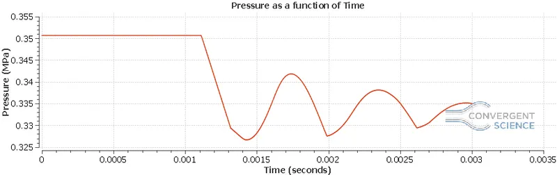
Development of Pressure in the Domain

Conclusion for pressure domain:

• The initial pressure difference between the two regions is 5 bar. As the mixing occurs, thepressure difference reduces in both regions.
• Initially, the pressure of N2 drops due to expansion and that of O2 rises due to compressionof the gas. Here we get the first instance of minima and maxima of the graph.
  After this, the shock wave gets reflected from the wall causing an increase in pressure. Andthis cycle gets repeated with diminishing values of maximum and minimum pressure.
• After every cycle, it can be seen that the high -pressure and low-pressure regions getinterchanged. To attain a steady-state, the simulation time should definitely be greaterthan 0.003 sec.

For Temperature

The temperature in High and Low-pressure zones (Region 0: High-pressure, Region 1:Low-pressure)

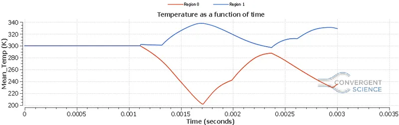
Temperature across the shock tube

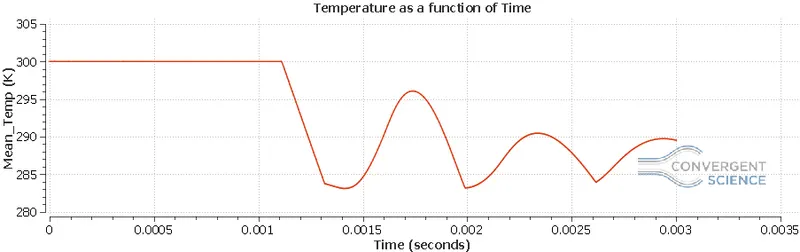
Conclusion for Temperature domain:

• A similar pattern of consecutive maxima and minima can be observed for temperature too.This is because the pressure is directly proportional to temperature.
• In High-pressure region, the temperature, initially starts to decrease and it is vice-versa for the Low-pressure region.

Development of Velocity in the Domain

Mass fraction of N2 in the Domain

Conclusion for velocity domain:

• Fluid passes through a shock wave, pressure, temperature, and density will increase; velocity will decrease.