Week 7: Shock tube simulation project
Aim: Perform a transient simulation of a shock tube using converge, plot the temperature and pressure history in the domain and cell count with time, Post process results using paraview.
The geometry used in the simulation.
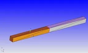
Setup-
Applications-
-Time-Based
Materials used-
Species-Air(O2,N2)
Simulation Parameters:
Run Parameter: Transient-state solver | Full Hydro. | Compressible
-Start time-0. End time-0.03 s
-Initial time step=minimum time step=1e-9 s
-Maximum time step=1 s
Max CFL limit(Convection/Diffusion): 1.0/2.0
Boundary conditions-
-High pressure walls-WALL- stationary, fixed, Slip, Temperature-300k, Zero Normal Gradient for Turbulent kinetic energy boundary condition
-Low pressure walls-WALL- stationary, fixed, Slip, Temperature-300k, Zero Normal Gradient for Turbulent kinetic energy boundary condition
-Front- 2D(high pressure and low pressure)
-Back - 2D(high pressure and low pressure)
Initial Conditions/Regions:
Region_O- High pressure region
-Pressure: 100000 pa
-Species- N2
Region_1-Low pressure region
-Pressure: 10000 pa
-Species-O2
Events:
0, High Pressure, Low Pressure, Close
0.001, High Pressure, Low Pressure, Open
Base Grid:
dx=dy=dz= 0.001m
Adaptive Mesh Refinement:
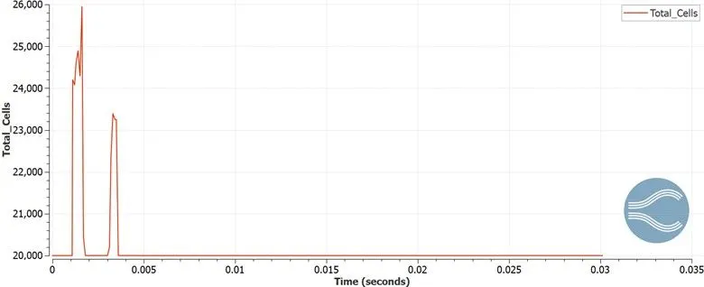
Pressure, Max-Embedding Level: 2, Sub-grid criterion-2.5, 25000 Max cells.
Mesh
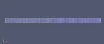
Total cells present in the geometry. The graph shows the total cells were close to 20000 and varied initially during the 0.001s time of opening events.
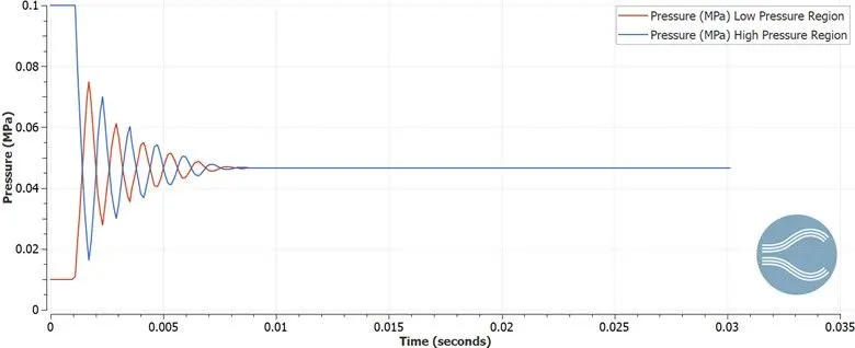
The pressure graph below shows the pressure from low pressure and high pressure regions.
It can be seen the pressure starts changing after 0.001s when diaphragm is opened. The pressure is increasing in the low-pressure region while it is decreasing in the high pressure. The up and down variation reflects pattern due to shock wave and it’s reflection.
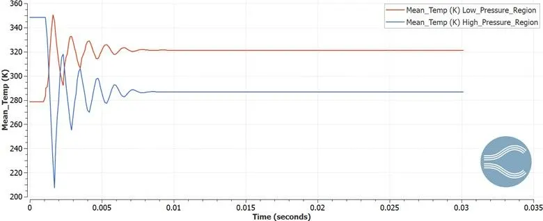
The temperature graph shows pattern similar to the pressure. It can be seen the temperature in high pressure region starts to decrease and temperature in low pressure region starts to increase. As the shock wave is produced and reflected back, the pattern continues until the low pressure region becomes constant at 320K and high pressure region reaches 285K.
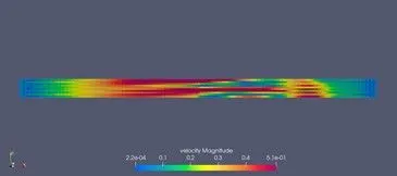
Velocity_Contour
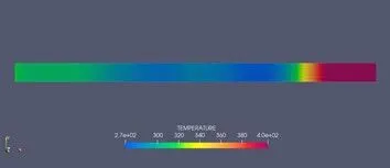
Pressure_Contour
Conclusion:
- A shock tube simulation was performed using converge.
- The temperature and velocity graphs were showing patterns affected by the shock wave and their values in high and low pressure region varies in opposite manner.
- The adaptive mesh refinement was used for better accuracy and understanding.
Youtube Animation Link: