Week 7 - Mid-term Project - Natural Convection
Mid-term Project - Natural Convection
Aim
To conduct thermal simulation of control panel at 25 deg.c and identify the temperature of the panel
Introduction
Natural convection occurs as a result of variations in fluid density above heated equipment. This density contrast induces fluid circulation, causing hot air to ascend while cold air settles on the heated surface. The Bousennesq approximation proves to be a highly accurate method for modeling this natural convection behavior.
Objective
- To establish the configuration of the control panel
- Mesh the system
- To conduct thermal simulation
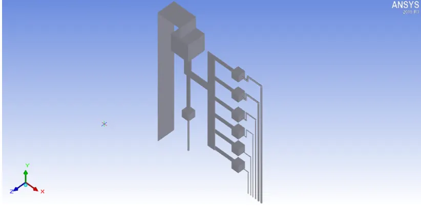
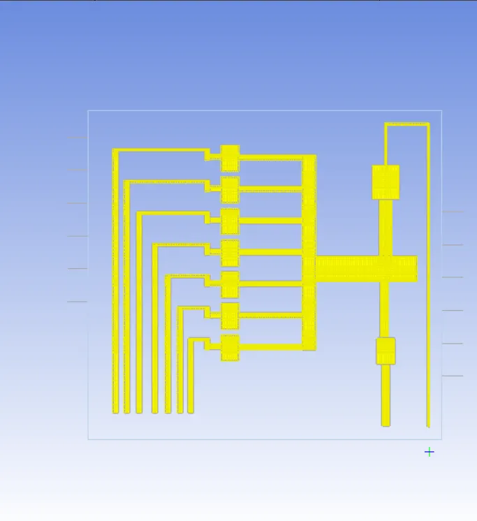
The geometry is created in accordance to the dimentions given in the problem statement
Meshing
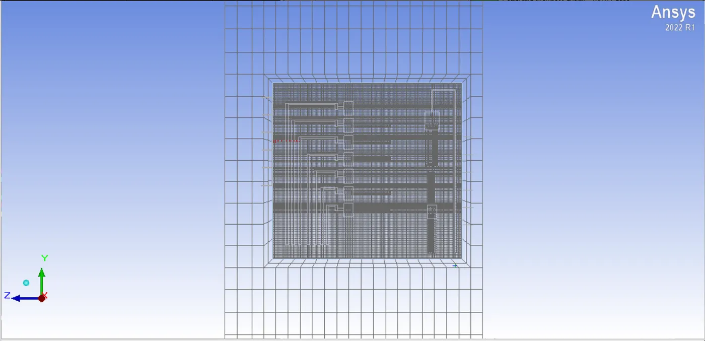
The provided image indicates that the generated mesh comprises 1518308 elements and 1571356 nodes. The accompanying images below depict the computational mesh on three mutually perpendicular planes, each passing through the center of the control panel.
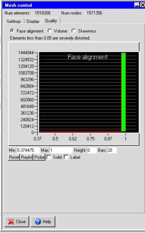
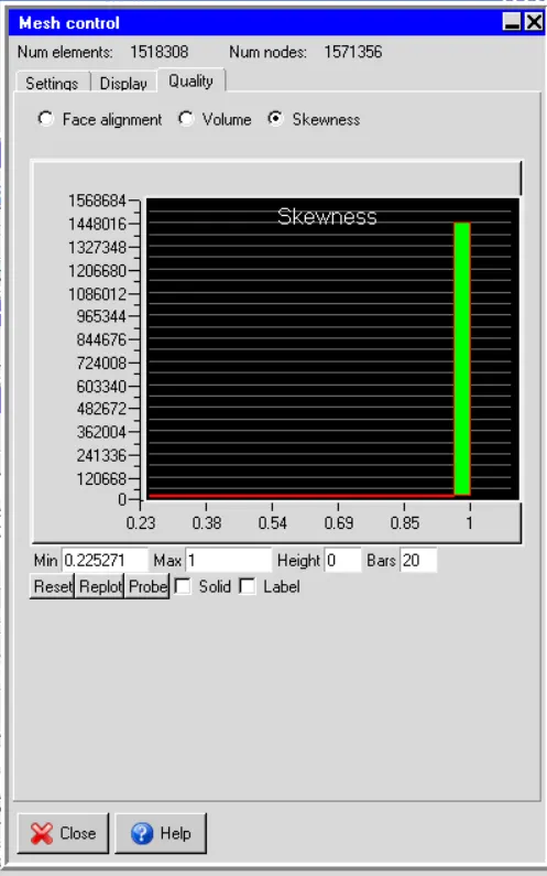
Mesh quality showed good quality meshes
Result
In this section, we delve into the simulation results.
Residuals:
Residuals for the following equations are graphed against the number of iterations:
i. Continuity equation
ii. X-Momentum equation
iii. Y-Momentum equation
iv. Z-Momentum equation
v. Energy equation
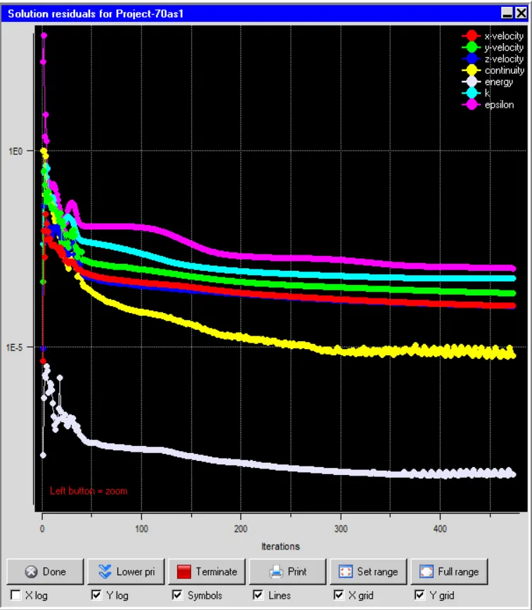
The plot reveals that the residuals exhibit minimal variation within the range of 100 to 500 iterations, suggesting that the solution has achieved a steady state. For the current project, simulation results post 500 iterations are deemed representative of the steady-state conditions.
Temperature
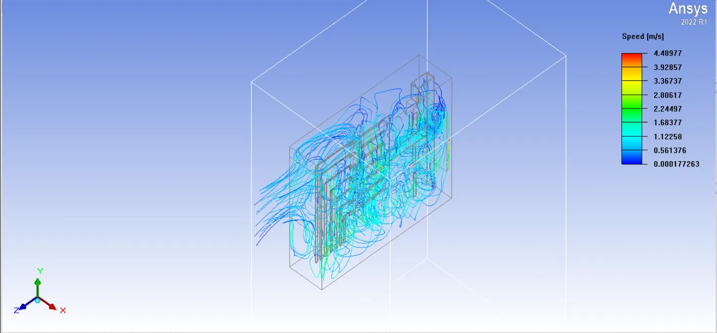
Velocity
Conclusion:
In this project, a low-voltage control panel model was meticulously designed in ANSYS Icepak, adhering to the provided design specifications. The meshing process incorporated non-conformal meshing and per-object meshing parameters within the Icepak mesher. The solver setup was configured to account for key physical phenomena, including Joule heating, natural convection, turbulence, and radiation heat transfer.
The Fluent solver in ANSYS Icepak was employed to solve the three-dimensional steady-state governing equations for flow and thermal fields across the computational domain. The simulation results lead to the following key conclusions:
i. Steady-State Results Confirmation:
Both the residual plot and the monitor plot collectively indicate that the simulation outcomes become stable after 500 iterations, establishing them as steady-state results.
ii. Velocity Contours Analysis:
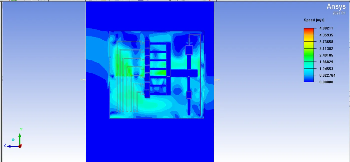
Examination of steady-state velocity contours reveals that the maximum air velocity within the computational domain is recorded at 2.7/s.
iii. Temperature Distribution:
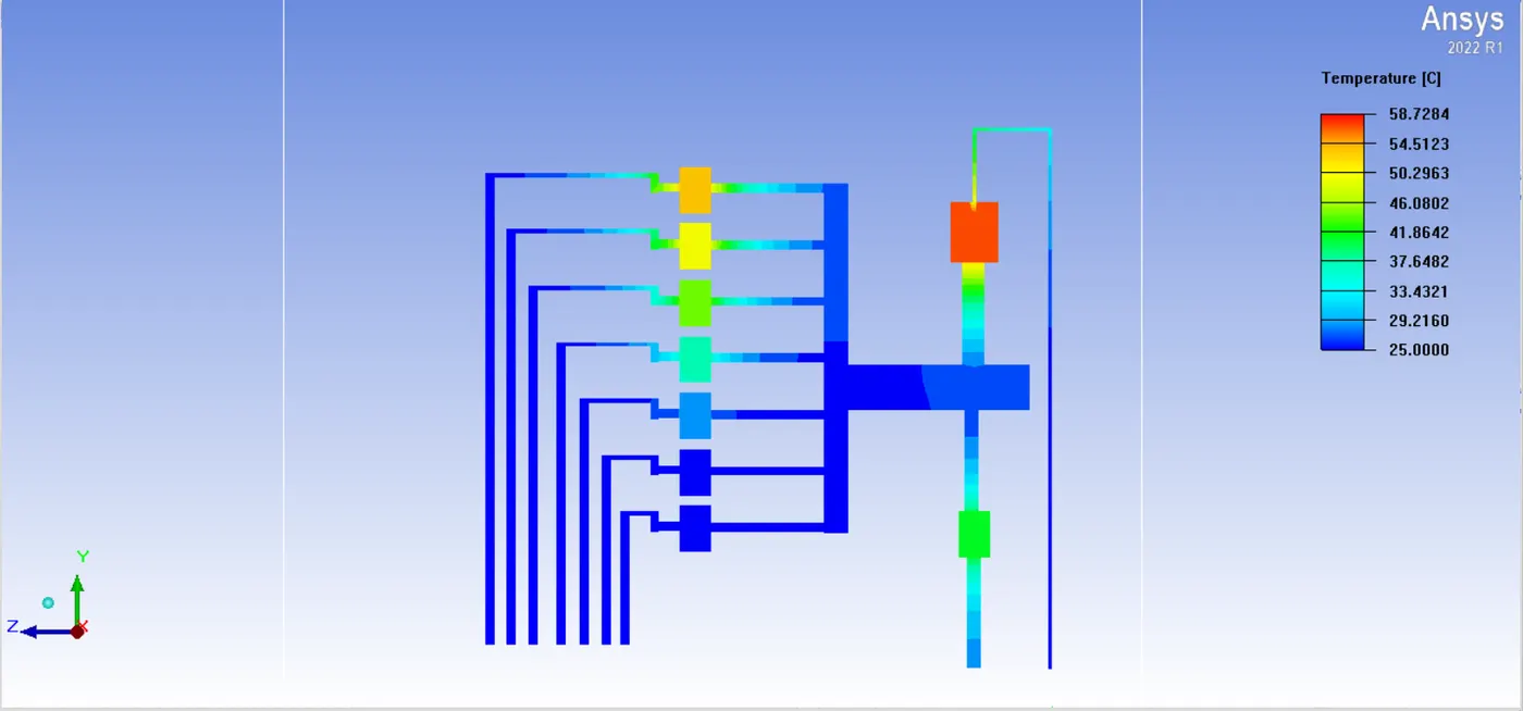
The highest steady-state temperature of 58.73°C is localized at the IG