Week-7 Head Impact

Skill-lync project report

Aim: The objective of this project is to simulate a typical crash scenario involving a pedestrian head and a car hood with the components provided and calculate the head injury coefficient (HIC). The scenario is to be modelled in three separate iterations. In the first iteration, the crash is to be modelled using the simple head model with the hood represented by a rigid wall. In the second iteration, the head model is to be replaced with the detailed head model provided. In the third iteration, the detailed pedestrian head is to be used along with the meshed hood model provided.

Case setup: The first keyword file provided consists of a simple head model. It is a sphere consisting of shell elements, as shown below.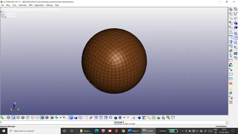

Figure 1: Simple pedestrian head model

It is to be modelled with a simple elastic material with the following material properties taken from the detailed head model: -

• Young’s modulus: 207 GPa
• Poisson’s ratio: 0.28
• Density: 2.906 X 10^-6 kg/mm³
• Shell thickness: 15 mm

The second keyword file contains a detailed variant of the pedestrian head, as illustrated below.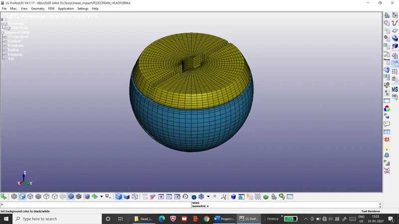

Figure 2: Detailed pedestrian head model

It is modelled with material, element and other relevant properties selected as per the vehicle regulation standards E/ECE/324/Rev.2/Add.126 decided by the United Nations economic commission of Europe (UNECE). The material properties are defined with the kg,mm,ms units.

The third keyword file consists of a meshed car hood, as shown below.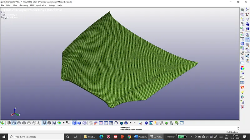

Figure 3: Meshed car hood model

It is to be modelled with a piecewise plastic material with the following properties of aluminium.

• Density: 2.68 X 10^-6 kg/mm³
• Young’s modulus: 75 GPa
• Poisson’s ratio: 0.33
• Yield strength: 0.075 GPa

The stress-strain curve of the material is to be defined as the following graph.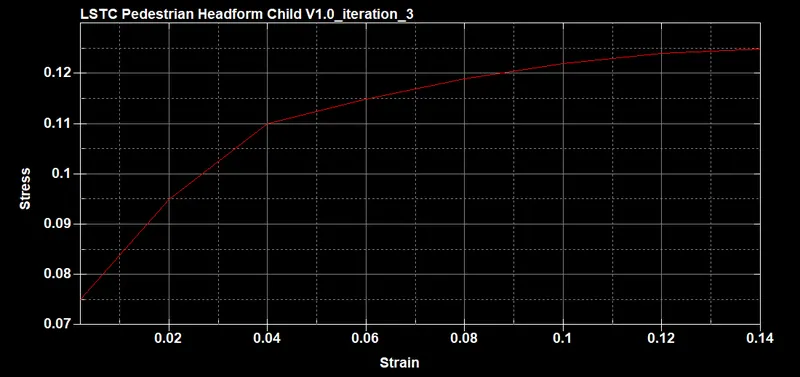

Figure 4: Aluminium stress-strain curve

Expected deliverables: The following outputs are expected from the project for all three iterations.

• Stress vs. strain plot for the head.
• Acceleration plot for the head.
• Head injury coefficient in all three iterations. Given by integrating acceleration of head over run time and using the result(I) in the following equation.

HIC = T*(I/T)^2.5 ;T=run time ,I=Integration of acceleration

Procedure: The various iterations are worked on through the following sequence of steps: -

1. The keyword file of the simple head model is imported into the LS-PrePost workspace.
2. The MAT>001-ELASTIC keyword is included to define the material for the head, as specified in the case setup. This material is assigned to the part.
3. The SECTION>SHELL keyword is modified so that element formulation of 16 (Fully integrated shell element) and shell thickness of 15 mm is specified for the shell elements. This section is then assigned to the part.
4. A rigid wall is defined with the following attributes to represent the car hood.

• Coordinates of normal vector’s tail: -500, 23, 785
• Coordinated of normal vector’s head: -499, 23, 790
• Friction coefficient: 0.8

5. The velocity of the head is defined by editing the INITIAL>VELOCITY keyword. The velocity magnitude is set as 10 mm/ms with an angle of impact of 50 degrees. Thus, the head model is assigned an x velocity of -6.427876 mm/ms and a z velocity of -7.6604444 mm/ms.
6. A self-contact is assigned to the head model via the CONTACT>AUTOMATIC_SINGLE_SURFACE keyword.
7. The CONTROL>TERMINATION keyword is edited so that run time 15 ms and minimum time step is 0.015 ms.
8. The DATABASE>BINARY_D3PLOT and DATABASE>ASCII_option keywords are edited so that the output animation has a minimum time step of 0.03 ms. The DATABASE>EXTENT_BINARY keyword is edited so that strain is recorded in the d3plot file.
9. The file is then run using the LS-Run solver.
10. The energy history is plotted and checked for discrepancies.
11. An element is selected at the point of impact and the stress history is plotted. This plot is output as an excel file. The strain history is also plotted and output in the same manner. These plots are combined in an X-Y plot to obtain the stress vs. strain plot.
12. A node at the opposite side of the point of impact is selected so that acceleration plot is generated from that node.
13. The acceleration plot is then integrated over the run time and the results are output as an excel file. The stable value here is then used to calculate HIC.
14. The detailed head model is imported into the LS-PrePost workspace as the second iteration.
15. The transform tool for elements is used to rotate the model by 40 degrees about the y axis to orient it to the proper position.
16. A rigid wall is defined with the following parameters.
    1. Coordinates of normal vector’s tail: -3, 3, -135
    2. Coordinated of normal vector’s head: -2, 3, -130
    3. Friction coefficient: 0.8
17. A velocity of 10 mm/ms is defined for the head model by the create entity tool.
18. The CONTROL>TERMINATION keyword is edited so that total run time is 15 ms and minimum time step is 0.015 ms.
19. The DATABASE>BINARY_D3PLOT, ASCII_option and EXTENT_BINARY keywords are added so that plots and animation have a time step of 0.03 ms and effective strain output.
20. The keyword file is then run in LS-Run.
21. The energy history is plotted and checked for discrepancies.
22. The stress and strain at an element in the skull region are plotted.
23. The acceleration at the centre of the head is plotted and integrated over the run time to obtain the HIC.
24. A copy of the second iteration’s keyword file is used as the third iteration, where the hood mesh is added.
25. The rigid wall is deleted from the model and the hood mesh is imported.
26. The MAT>24-PIECEWISE_LINEAR_PLASTICITY keyword is added and assigned to the hood.
27. A shell section is assigned to the hood with element formulation of 16 (fully integrated shell element) and thickness of 5 mm.
28. Fixed constraints are added to the hinge and latch regions of the hood by the create entity tool, as shown below.

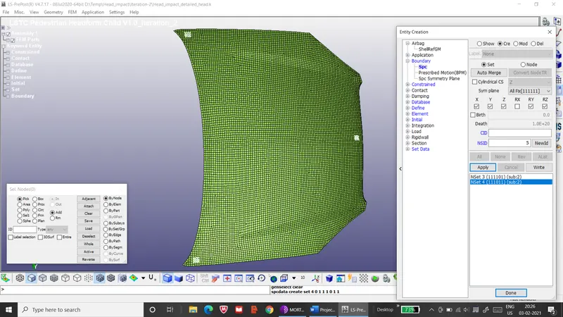Figure 5: Hinge and latch constraints on hood

29. Self-contact is defined for the hood by the CONTACT>AUTOMATIC_SINGLE_SURFACE keyword.
30. The CONTACT>AUTOMATIC_NODES_TO_SURFACE keyword is edited to establish contact between the head model and the hood.
31. The file is then saved and simulated in LS-Run.
32. The energy plot is checked for discrepancies.
33. The stress vs strain is plotted at the area of impact for both the head and the hood.
34. The acceleration plot is obtained from the acceleration node. The plot is then integrated over the run time and the result is used to compute the HIC.

Results: The following results are obtained from the various iterations: -

1. Iteration 1: In this iteration, the simple head model was used with a rigid wall representing the hood. The energy plot obtained here is illustrated below.

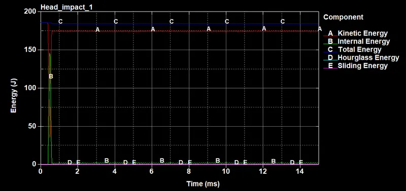Figure 6: Energy plot for first iteration

It shows a slight drop in total energy during impact. This discrepancy could not be eliminated despite optimal element formulation and hourglass control.

The stress vs. strain curve at the point of impact is shown below.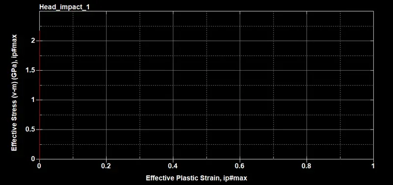

Figure 7: Stress vs. strain curve for first iteration

For unknown reasons, the strain in the model was not captured, despite the inclusion of the ENTENT_BINARY keyword in the database.

The acceleration in the head model is shown below.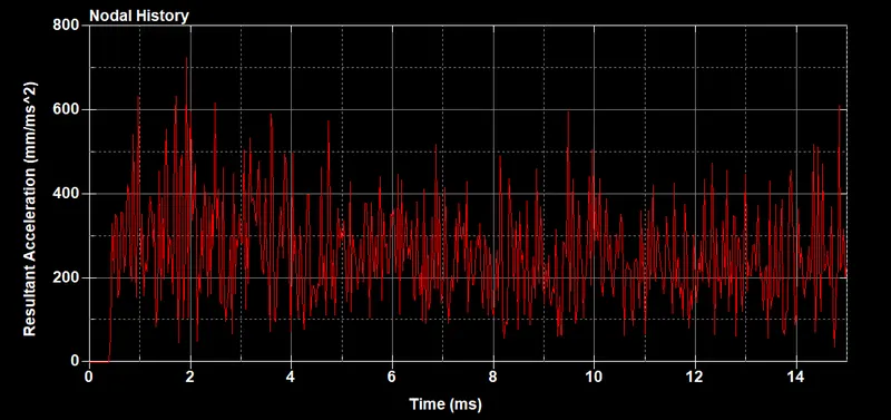

Figure 8: Acceleration plot for first iteration

It shows persistent vibrations in the head due to the simple elastic nature of the material used. The lack of a plastic behaviour ensures that the vibrations are not dampened.

The integration plot for the acceleration is shown below.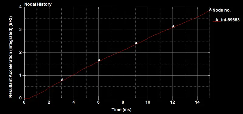

Figure 9: Integration plot of acceleration for first iteration

It never reaches a steady value due to the persistent vibrations. Ultimately the maximum value of 3850 is chosen along with time range of the entire run time i.e., 15 ms. Using these in the formula, the HIC is computed to be 15831240. This value is clearly much higher than the permissible value of 1000 specified by the UNECE standard. However, based on the acceleration plot and the nature of the simulation, this value is not representative for any generic head impact test. The inaccurate material selection, simplistic modelling of the head & hood and the observation of persistent vibrations contribute to the divergence from realistic values.

2. Iteration 2: In this iteration, the head model is a detailed model of the typical head impact measuring instrument. The hood is still modelled as a simple rigid wall. The energy plot from the simulation is shown below.

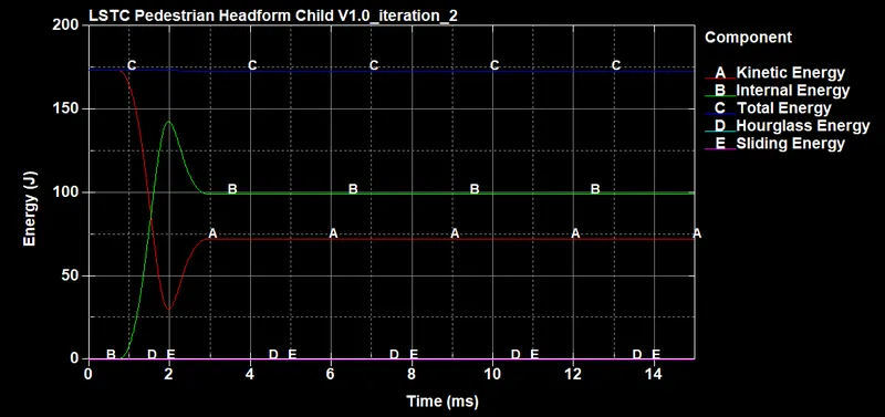Figure 10: Energy plot for second iteration

Unlike the first iteration, there is no drop in total energy. This can be attributed to better material selection and element formulation.

The stress vs. strain plot at the point of impact is illustrated below.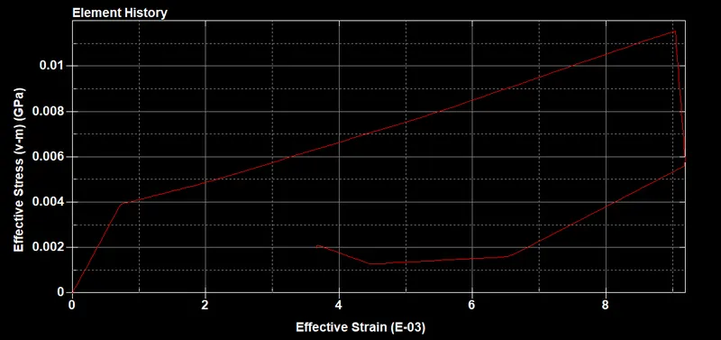

Figure 11: Stress vs. strain curve for second iteration

It shows a clear hysteresis in the hyper-elastic material used for the skin section of the head, along with a residual stress that remains after impact.

The acceleration recorded at the centre node is plotted below.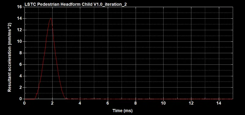

Figure 12: Acceleration plot for second iteration

Unlike the first iteration, the acceleration plot here shows no vibrations in the head model after impact. The hyper-elastic material dampens any vibrations. The entirety of the acceleration recorded happens during the moment of impact. After integrating the acceleration over run time, the following plot is obtained.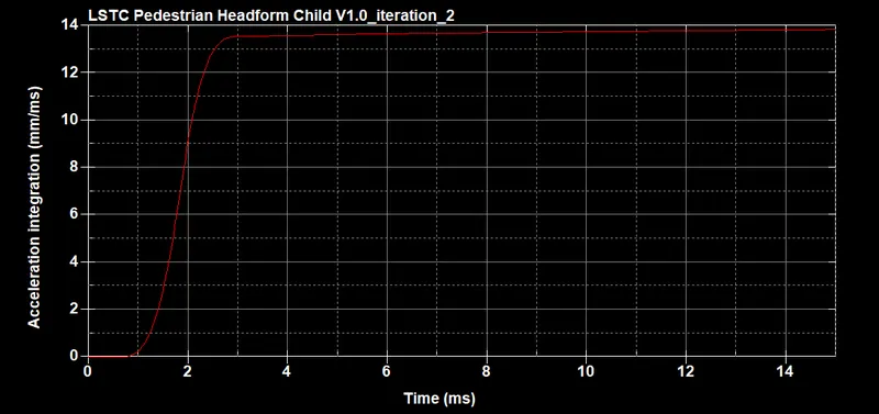

Figure 13: Integration of acceleration for second iteration

In this iteration, the integrated value reaches a steady state at 13.8 mm/ms. The value of time interval can be taken as 2 ms. With these values, the computed value of HIC is 250. This value is substantially lower than the value seen in the first iteration. This can be attributed to the material used for the skin region of the head and the limitation of acceleration to moment of impact.

3. Iteration 3: This iteration contains the detailed head model as well as the meshed hood model, rather than the rigid wall. The stress vs. strain plot for the head region at the point of impact is shown below.

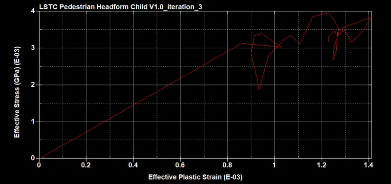Figure 14: Stress vs. strain curve for head in third iteration

It shows a lot of irregularities, but there is a barely discernible curve that shows strain hardening.

The stress vs. strain plot for the hood at the point of impact is illustrated below.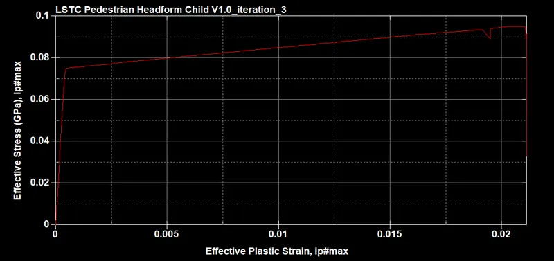

Figure 15: Stress vs. strain curve for hood in third iteration

It is an exact replica of the stress-strain curve that was defined for the hood material. Had the time step in the d3plot been smaller, the piecewise linearity of the plot would have been visible.

The acceleration recorded for this iteration is shown below.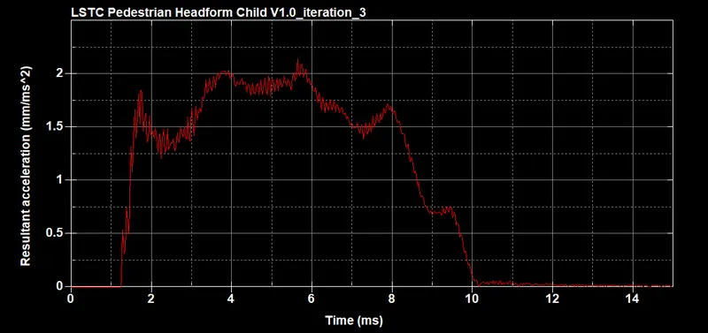

Figure 16: Acceleration plot for third iteration

It shows an extended period of impact, as well as a reduced magnitude of maximum acceleration. This confirms the effectiveness of a deformable hood in reducing head impact, as opposed to a hard & rigid one. Upon integrating, the steady value is 13 and the time period for the impact is about 9 ms. Thus, the resultant HIC is computed to be about 23. This is the lowest value of HIC in all the various iterations. This provides even stronger evidence that a deformable hood is better at reducing head impact than a rigid one.

Conclusion: The head impact scenario was successfully simulated in successive iterations. These simulations verified the importance of a proper head model for accuracy of results and the importance of a deformable hood for reduction of impact severity.