Week-7 Head Impact

PEDESTRIAN HEAD IMPACT SIMULATION USING LS-DYNA

AIM:

To perform the Head Impact Simulation and calculate the Head Impact Criterion (HIC) value for the following cases.

1. Simple head model impacting against a rigid wall
2. Child head form dummy model impacting against a rigid wall
3. Child head form dummy model impacting against the hood

PROCEDURE:

Case (1): Simple head model impacting against the rigid wall:

The given LS-Dyna keyword file of the simple head FE model is opened in LS-PrePost using the option File>Open>LS-Dyna Keyword File.

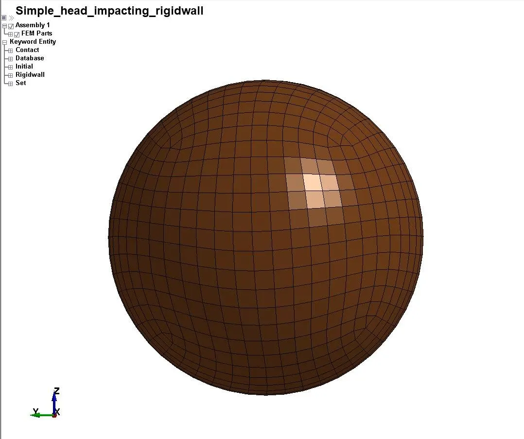
Fig.2. FE model of simple head

1. Part definition

Section properties:

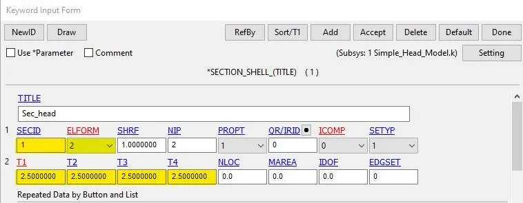
Fig.3. Section property of simple head.

The section properties of the simple head are assigned as shell element with 2.5 mm thickness and ELFORM=2, Belytschko-Tsay element formulation.

Material properties:

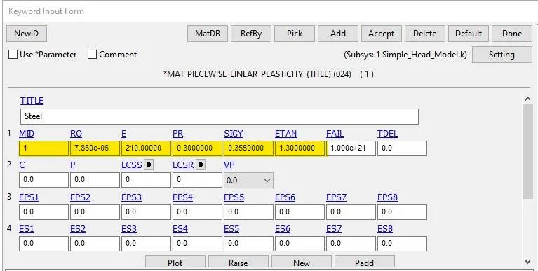
Fig.4. Material property of simple head.

MAT24 (Piece wise linear plasticity) material card is used to assign the steel material properties to the simple head model. The MAT24 represent Piecewise linear isotropic plasticity. With this material model it is possible to consider the effect of the strain rate.

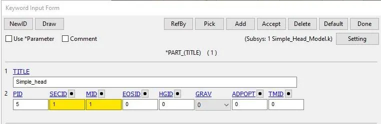
Fig.5. Part details of simple head model.

2. Boundary condition

Initial velocity:

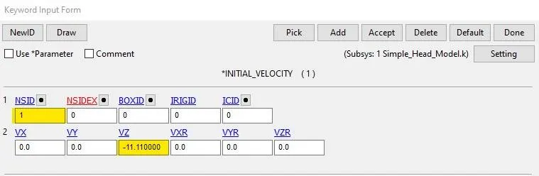
Fig.6. Initial velocity

The simple head model is assumed to be impacting the rigid wall at a velocity of 40 km i.e. 11.11 mm/ms in negative Z-direction towards the rigid wall.

Rigid wall planar:

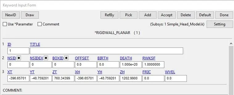
Fig.7. Rigid wall planar.

The rigid wall is created at a distance of 15 mm from the bottom of the simple head model.

Contact details:

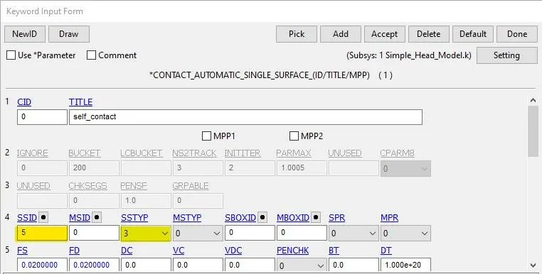
Fig.8. Contact between simple head model and rigid wall

The contact type selected is AUTOMATIC_SINGLE_SURFACE. It is quite helpful to apply this contact method in the crash models because all the elements are included in one single set and LS-DYNA considers also when a part comes into contact with itself. The FS and FD are static and dynamic friction coefficient with a value of 0.02 is entered in the contact card. The simple headform model is the slave(SSID=5).

3. Control and Database options:

Control function:

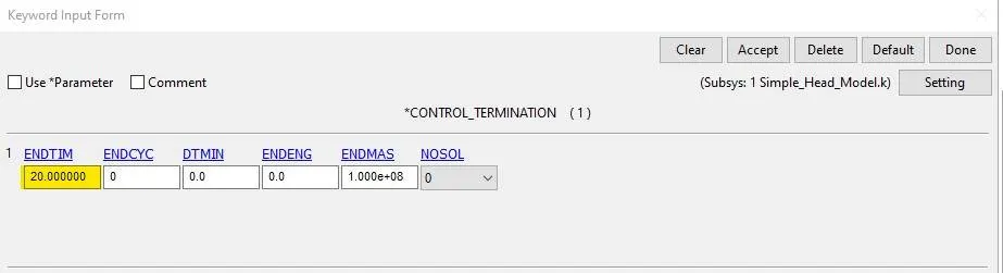
Fig.9. Control termination

The control termination function is enabled to specify the end time of the simulation. The termination time is set for 20 ms.

Database options:

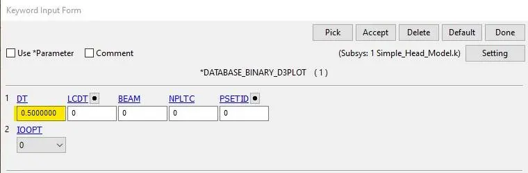
Fig.10. Database binary D3plot.

The time step value of 0.5 ms is given for the BINARY_D3PLOT and DATABASE_ASCII options for GLSAT, NODOUT and RWFORC

DATABASE_EXTENT_BINARY card with STRFLG =1, is used to compute the elastic strain in the model.

DATABASE_HISTORY_NODE card is used to compute the HIC value of a 688991 node in the model.

The keyword file created is checked for errors using the option keyword manager>model check. The keyword file is saved using ‘.k’ extension and is made to run in the solver by getting normal termination message.

Case (2): Child headform dummy model impacting against the rigid wall:

1. Part definition

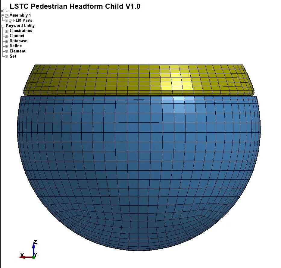
Fig.11. Imported FE model of dummy child headform.

The standard dummy model of child headform was provided with the necessary keywords for impact simulation as shown in fig. 11.

For case (2) impact simulation, the provide standard dummy model of child headform has to be rotated about 50⁰ along the Y-axis to replicate the Euro NCAP impact simulation as shown in fig.1, by pulling it into a new keyword file created by LS-PrePost by using *DEFINE_TRASFORMATION and *INCLUDE_TRANSFORM as shown in fig.12 and fig. 13.

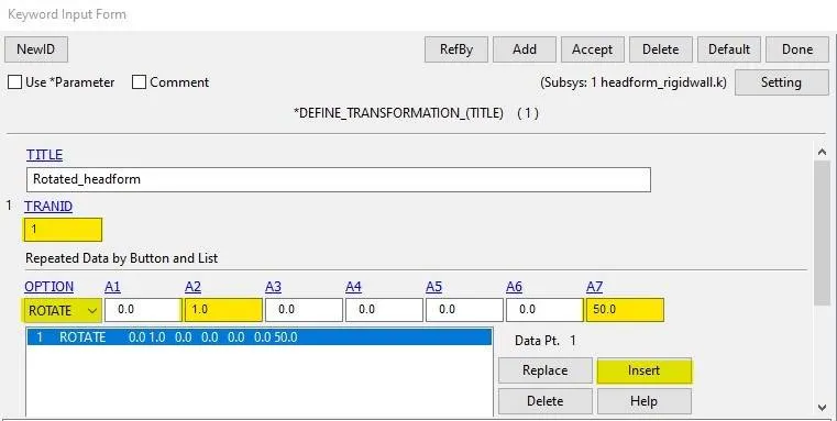
Fig.12. Define a transformation card to rotate the child's headform.

Using the DEFINE_TRANSFORMATION card with TRANID=1, the dummy headform model is rotated by OPTION>ROTATE along Y-axis (A2=1) by 50⁰ (A7=50).

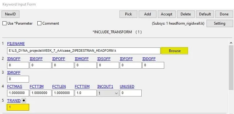
Fig.13. Include transform card.

INCLUDE_TRANSFORM card is used to pull the rotated standard dummy headform model file to the main file. The main file is saved with ‘.k’ extension.

Note: Filenames and pathnames are limited to 236 characters spread over up to three 80-character lines.

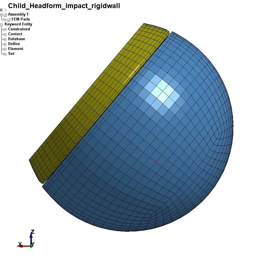
Fig.14. Child headform rotated at 50⁰ along Y-axis.

The main file is opened in LS-PrePost as shown in fig. 14 to add the necessary keywords to complete the simulation setup.

2. Boundary condition

Initial velocity:

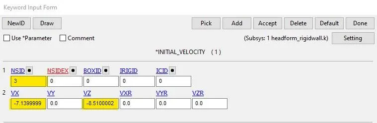
Fig.15. Initial velocity.

As per Euro NCAP standards, the initial velocity is taken as 40 kmph i.e, 11.11 mm/ms at an angle 50⁰. The vertical and horizontal components of the velocities are -7.14 mm/ms and -8.51 mm/ms respectively.

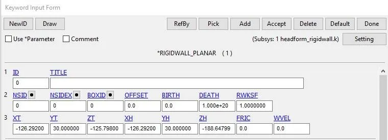
Fig.16. Rigid wall planar.

The rigid wall is created at a distance of 15 mm from the bottom of standard dummy headform model.

Contact details:

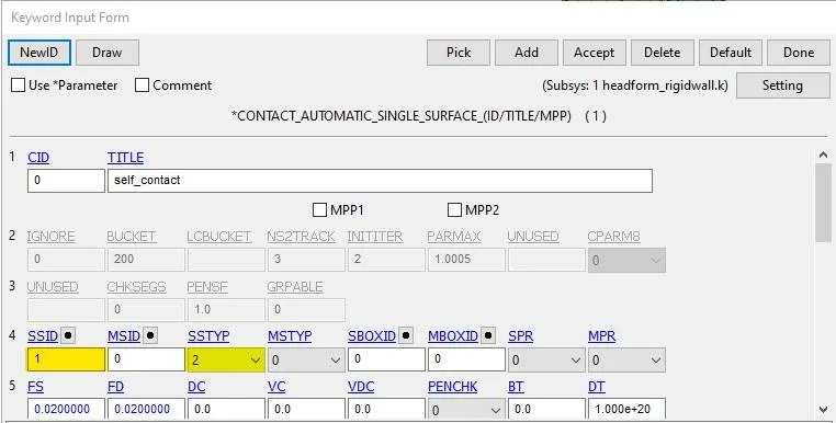
Fig.17. Contact between child headform model and rigid wall.

CONTACT_AUTOMATIC_SINGLE_SURFACE card is used to define contact between the rigid wall and dummy child headform model. The child headform model is taken as a slave (SSID=1).

3. Control and Database options:

Control function:

The termination time is set for 20 ms.

Database options:

The time step value for the BINARY_D3PLOT and DATABASE_ASCII option for GLSAT, NODOUT and RWFORC is given as 0.5 ms.

DATABASE_EXTENT_BINARY card with STRFLG =1, is used to compute the elastic strain in the model.

DATABASE_HISTORY_NODE card is used to compute the HIC value of a 25679 node in the model.

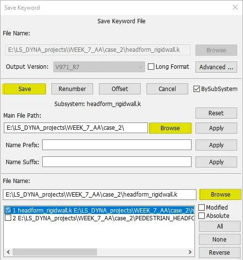
Fig.18. Keyword saving option.

The keyword file created is checked for errors using the option keyword manager>model check. The keyword file is saved to main file using the ‘save keyword as’ option as shown in fig. 18. The main file is made to run in the solver by getting a normal termination message.

Case (3): Child headform dummy model impacting against hood:

1. Part definition

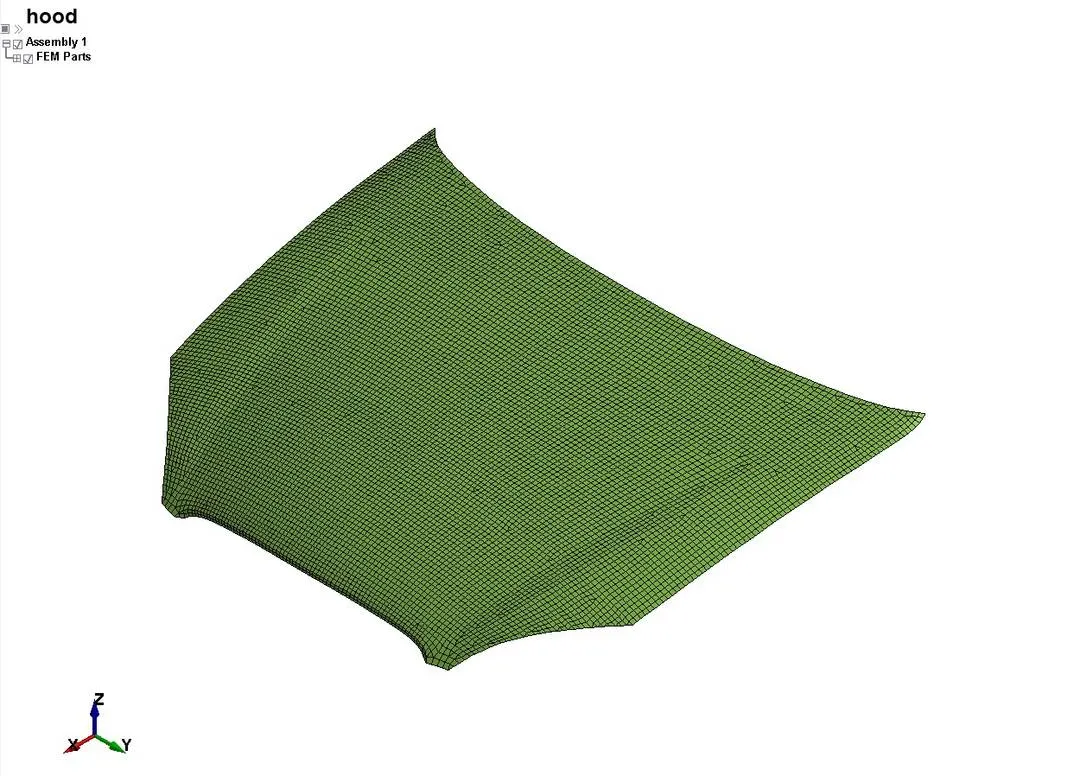
Fig.19. Imported FE model of the hood.

Section properties:

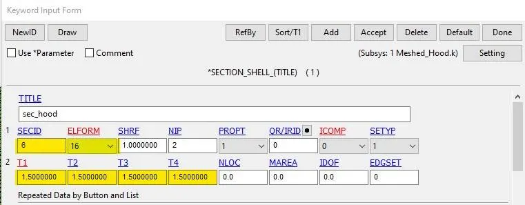
Fig.20. Section property.

The section properties of the hood are assigned as shell element with 1.5 mm thickness and ELFORM=16, Fully integrated shell element (very fast).

Material properties:

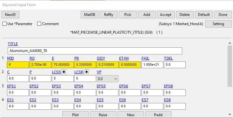
Fig.21. Material property of hood

MAT24 (Piecewise linear plasticity) material card is used to assign the Aluminium material properties to the hood. The MAT24 represents Piecewise linear isotropic plasticity. With this material model, it is possible to consider the effect of the strain rate.

The keyword file of the hood is saved using ‘.k’ extension. The keyword file of the hood is pulled into the main file using keywords *INCLUDE as shown in fig.22. The child headform is pulled into the main file by using keywords *DEFINE_TRASFORMATION and *INCLUDE_TRANSFORM which is similar to the case (2) scenario.

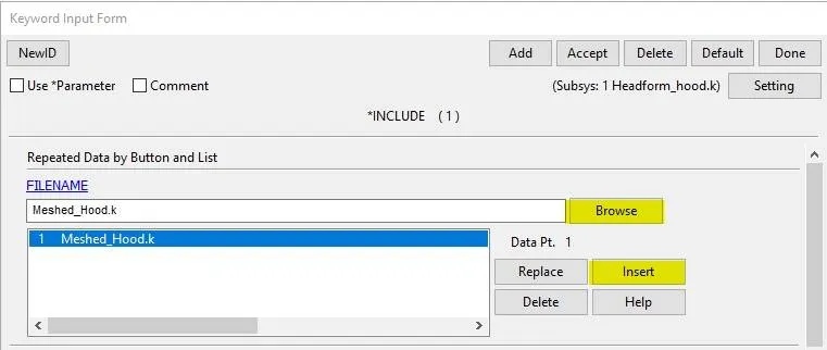
Fig.22. Include keyword.

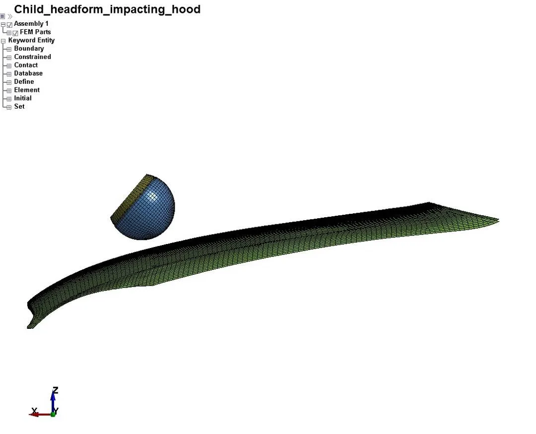
Fig.23. Main keyword file showing child headform and hood.

The main keyword file is opened in LS-PrePost as shown in fig. 23 to add necessary keywords to complete the impact simulation setup.

2. Boundary condition

Initial velocity:

As per Euro NCAP standards, the initial velocity is taken as 40 kmph i.e, 11.11 mm/ms at an angle 50⁰. The vertical and horizontal components of the velocities are -7.14 mm/ms and -8.51 mm/ms respectively.

Boundary SPC:

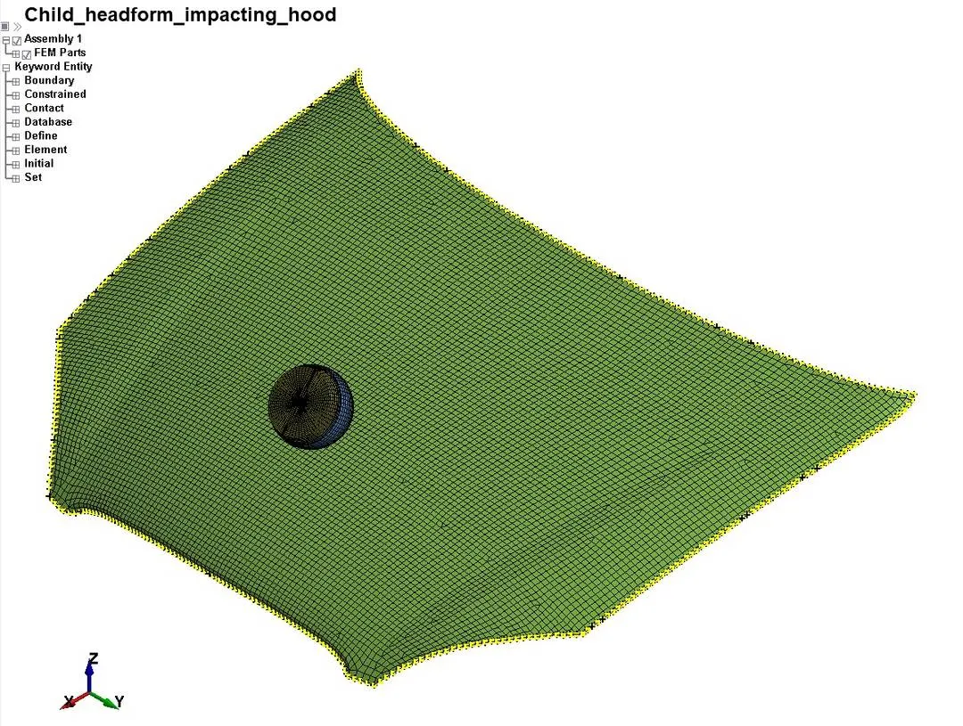
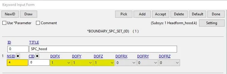
Fig.24. Boundary SPC card.

Using create entity option the nodes on the outer edges of the hood is selected and constrained all the translational motion using option boundary SPC set.

Contact details:

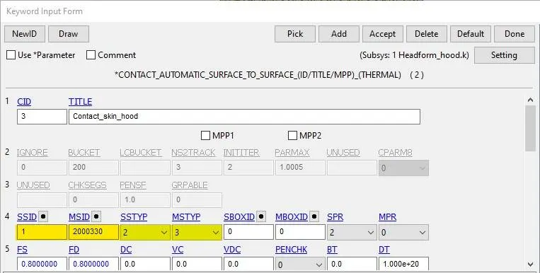
Fig.25. Contact details between hood and child headform.

CONTACT_AUTOMATIC_SURFACE_TO_SURFACE card is used to define contact between hood and dummy child headform model. The child headform model is taken as slave and hood as master. The FS and FD that are static and dynamic friction coefficient with a value of 0.8 is entered in the contact card.

Note: Increasing the value of FS and FD also increases the value of HIC, hence choose appropriate value for FS and FD.

3. Control and Database options:

The control card and database cards are same as that of case (2) scenario.

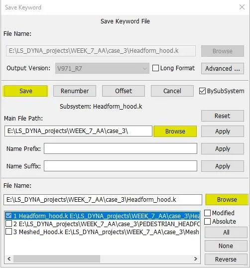
Fig.26. Keyword saving option.

The keyword file created is checked for errors using the option keyword manager>model check. The keyword file is saved to main file using ‘save keyword as’ option as shown in fig. 26. The main file is made to run in the solver by getting a normal termination message.

RESULTS:

The D3plot output file is opened in LS-PrePost using option File>open>LS-Dyna binary plot.

1. The animation of Von-Mises stress and Effective plastic strain contour is as shown below.

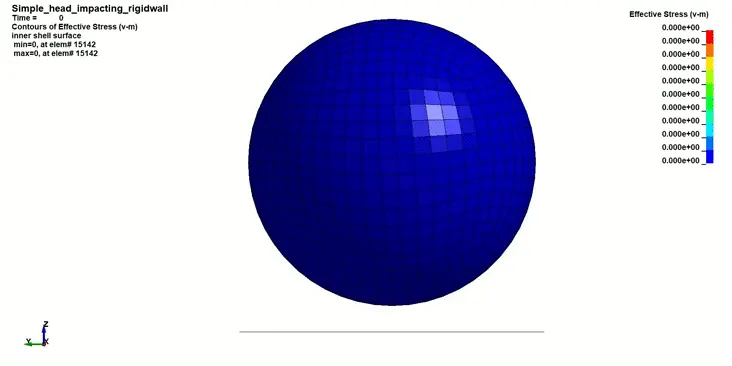
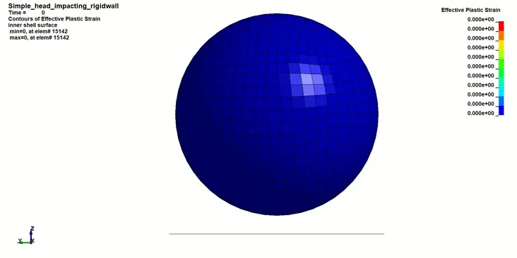
v-m stress contour for case (1) Effective plastic strain contour for case (1)

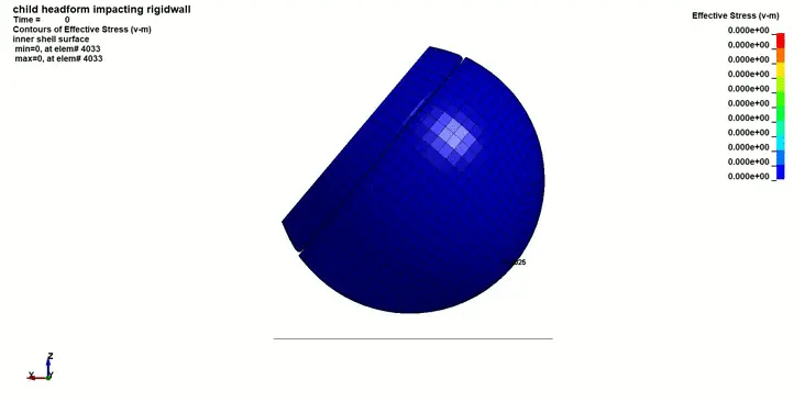
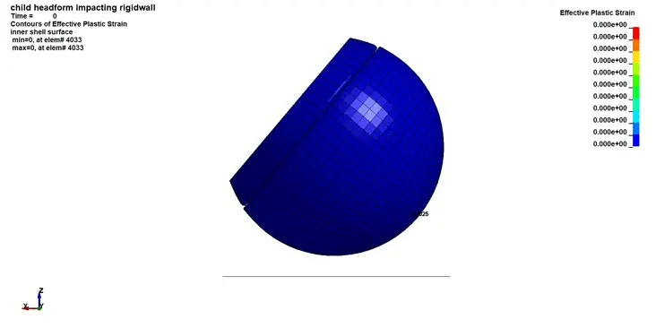
v-m stress contour for case (2) Effective plastic strain contour for case (2)

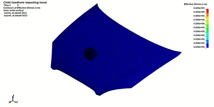
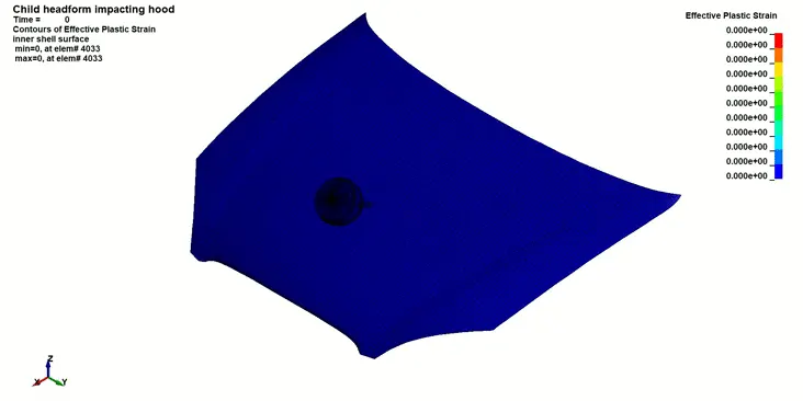
v-m stress contour for case (3) Effective plastic strain contour for case (3)

2. Stress plots

v-m stress plot for an element:

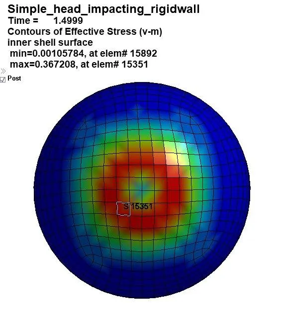
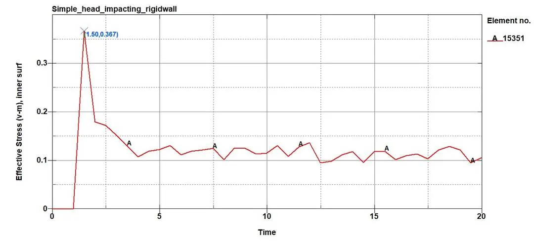
Fig.27 v-m stress plot for case (1)

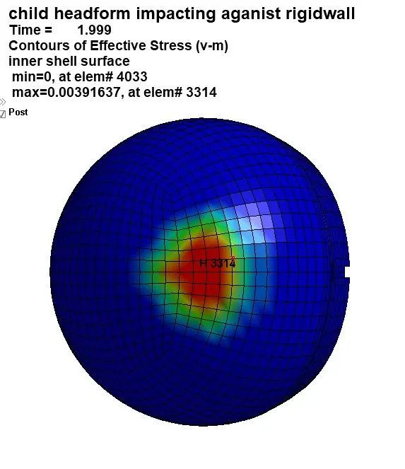
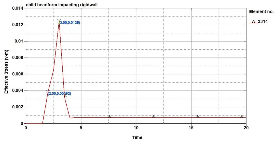
Fig.28 v-m stress plot for case (2)

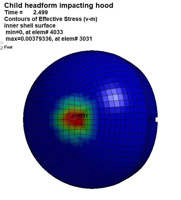
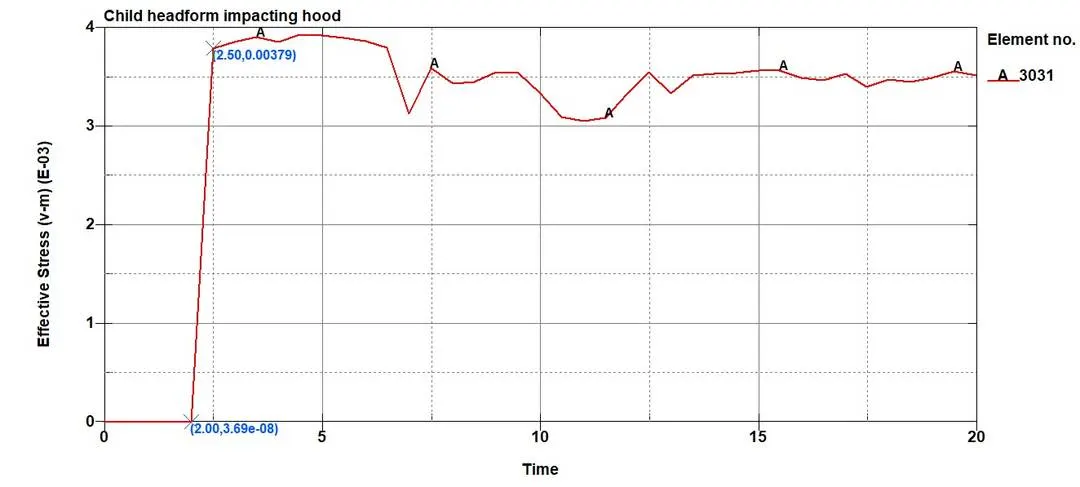
Fig.29 v-m stress plot for case (3)

In the first case, during the instant of impact, the maximum v-m stress developed is 367.2 MPa in the element 15351 which is beyond the yield stress value of 355 MPa.

In the second case, during the instant of impact, the maximum v-m stress developed is 3.916 MPa in the element 3314 and reaches a peak value of 12.5 MPa at 3 ms, and later the value of v-m stress reduces due to the bouncing back of the headform from the rigid wall.

In the third case, during the instant of impact, the maximum v-m stress developed is 3.793 MPa in the element 3031 and later it fluctuates steadily until the headform bounces back from the hood.

The v-m stress induced in the element for the third case is less compared to the second case because the hood gets deformed due to the impact and absorbs the energy, unlike the rigid wall which does not get deformed during impact.

3. Head Injury Criteria (HIC₁₅)

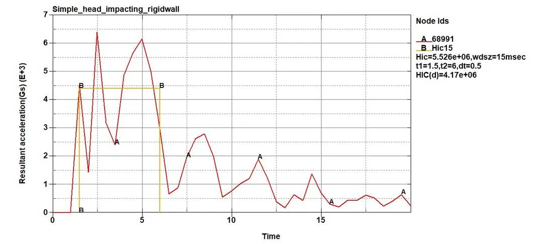
Fig.33 The resultant acceleration plot with HIC₁₅ value for case (1)

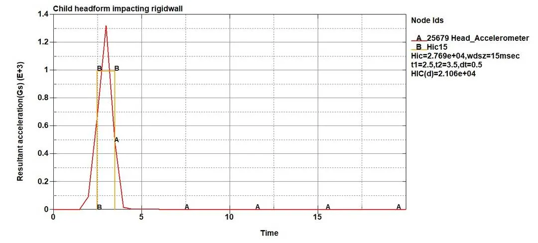
Fig.34 The resultant acceleration plot with HIC₁₅ value for case (2)

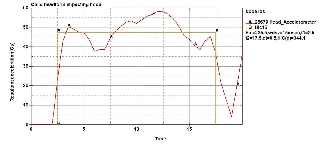
Fig.35 The resultant acceleration plot with HIC₁₅ value for case (3)

From the plot, the HIC₁₅ value for the first and second cases is beyond the safe value because the head model is impacting a nondeformable rigid wall. The HIC₁₅ value obtained from LS-PrePost for the third case is 235.5 and HIC_(d) value is 344.1 which is less than the safe HIC value of 650 as per Euro NCAP Protocol because the hood absorbs the impact energy and gets deformed.

Manual calculation of HIC value:

The expression to calculate the HIC value is,

HIC=maxt1,t2{[1t2−t1∫t2t1a(t)dt]2.5(t2−t1)}HIC=maxt1,t2⁡{[1t2-t1∫t1t2a(t)dt]2.5(t2-t1)}

From the plot,

The average value of acceleration for the time interval of t₁=2.5 ms and t₂=17.5 ms is, [1t2−t1∫t2t1a(t)dt]=48[1t2-t1∫t1t2a(t)dt]=48

Therefore, HIC=maxt1,t2{[48]2.5(17.5−2.5)}=239.438HIC=maxt1,t2⁡{[48]2.5(17.5-2.5)}=239.438

HIC(d)=0.75446(Free Motion Headform HIC)+166.4=0.75446×239.438+166.4=347.046HIC(d)=0.75446(Free Motion Headform HIC)+166.4=0.75446×239.438+166.4=347.046

The HIC₁₅ value obtained from LS-PrePost for the third case is 235.5 and HIC_(d) value is 344.1. The HIC₁₅ value obtained from the manual calculation for the third case is 239.438 and HIC_(d) value is 347.046. There is a small variation in the HIC value obtained from LS-PrePost and manual calculation which is acceptable.

CONCLUSION:

1. The impact simulation of pedestrian headform is created for a simple case scenario to a complex real-time scenario i.e.,

case (1): Simple head model impacting against rigid wall

case (2): Child headform model impacting against a rigid wall

case (3): Child headform model impacting against the hood.

2. The computational time required for the simple case is less compared to the real-time case scenario but the accuracy of the results is poor for a simple case.

3. There is a variation in the values for stress/strain and HIC₁₅ for all the cases because of the difference in material properties and boundary conditions.

4. The HIC₁₅ value obtained for case 3 was within the standard safe HIC₁₅ value of the EURO NCAP protocol.

Google Drive Link: Pedestrian head impact simulation