Week 7 - CHT Analysis on a Graphics card
The aim of this assignment is to mesh the given geometry in a coarse, base line mesh and then with a finer mesh to set-up an accurate simulation to perform conjugate heat transfer analysis on the provided geometry of a graphics card.
Geometry set-up:
The graphics card is further made up three main components:
The Processor:
Made of silicon and is the source of heat in this problem.

Its power dissipation is taken to be 95watts.
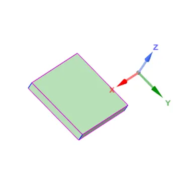 (The dimensions are 80mmX80mmX1mm.)
Therefore, the power density of this as a heat source would be 1.484375 X 10^9 W/m^3.
The processor is traditionally made out of silicon.
The Base:
The base (printed circuit board) is usually made out of an epoxy material known as FR4.
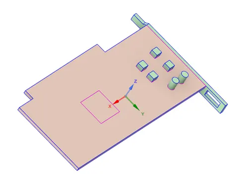
The base has all the components soldered onto it. Its body is non-conduction with conducting pathways etched onto it to complete circuits.
Aluminium Fins:
Its purpose is to conduct the heat away from the processor and the base and to dissipate it to its surroundings.
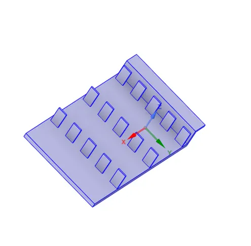
The tree of the geometry:
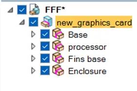
The “new_graphics_card” file that housed all of the components was chosen and in the ‘Analysis’ section, the ‘Share Topology’ was set to share.
Then, in the ‘Workbench’ tab, ‘Sharing’ section, the ‘Share’ option was chosen.
This enabled all the components to share their topologies and create effctive interfaces so that a conforming mesh is obtained across all the zones.
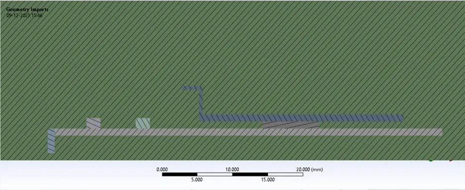
(Cut plane in the meshing interface with hatch patterns to demonstrate that no interference is occurring amongst components.)
Then, we move on to the meshing interface.
For a base line mesh, the default element size was taken.
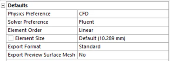

(Mesh details and statistics.)
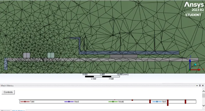
(The mesh analysed from a cut plane along the centre of the enclosure. The mesh is conforming across all the components. The mesh metrics are also attached in the same snippet.)
The steady-state solver was chosen as only the steady state temperature distribution needed to be analysed.
The ‘Energy’ box was checked. From the viscous turbulence models, the k-epsilon (standard) model was chosen.
Then in the ‘Materials’ dialogue box, the following materials were chosen/created:
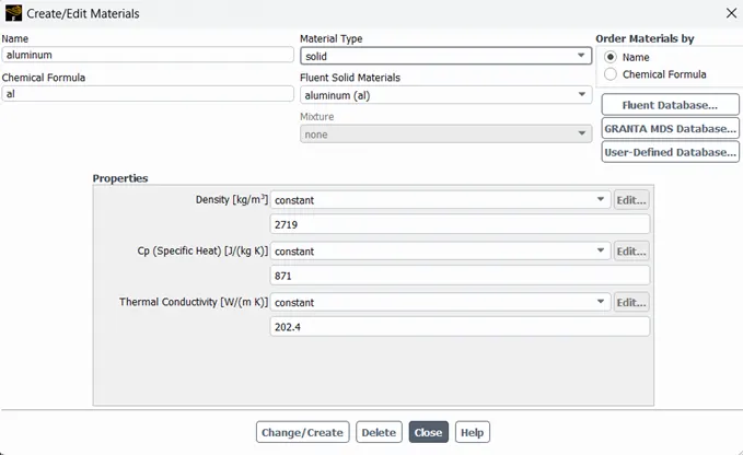
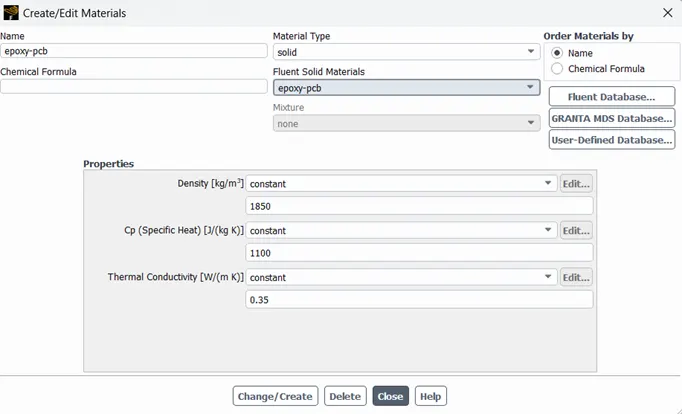
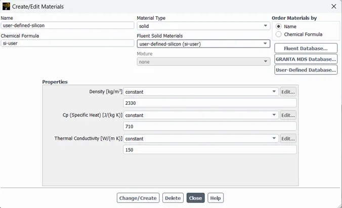
The fluid in the enclosure was taken to be air.
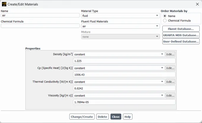
In the ‘Cell Zones’ option in the ‘Physics’ tab, these materials were appropriately assigned to the cell zones. The appropriate materials were also assigned in the ‘Cell Boundaries’ option.
At the ‘Inlet’ cell boundary, the velocity (Magnitude, Normal to Boundary) was set to be 5m/s.
The temperature of the inlet stream was set to be 300K.
Contours were created to show the surface temperature distribution on the graphics card. Animations were also created to record these contours.
The solution was then initialised (hybrid mode) and then run for 500 iterations.
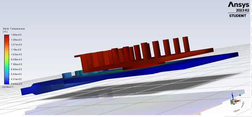
(Temperature contour.)
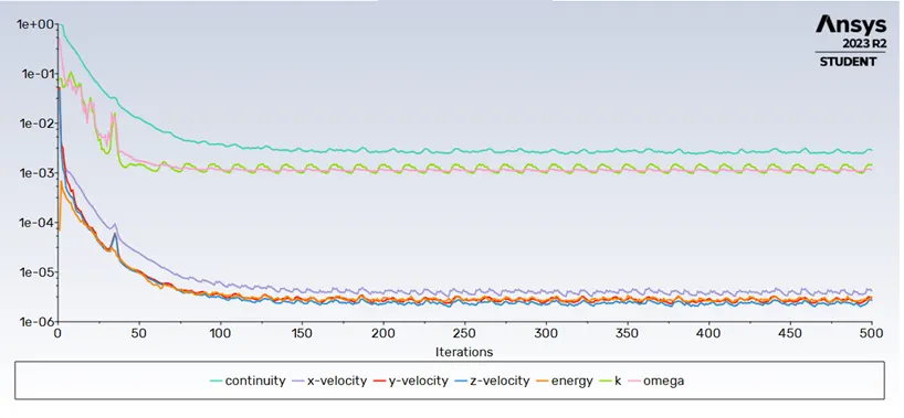
(Scaled Residuals.)
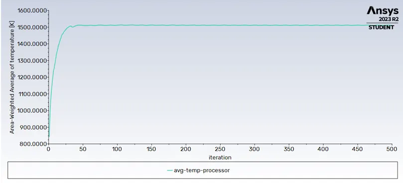
(Area-weighted average of surface temperature of the processor.)
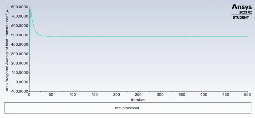
(Area weighted average of heat transfer coefficient of the processor.)
Computed value of the heat transfer coefficient (area weighted average) was 486.66336 Wm^-2K^-1.
Computed value of the surface temperature (area weighted average) was 1510.3653K.
The maximum temperature on/in the processor was computed to be 1513.5359K.
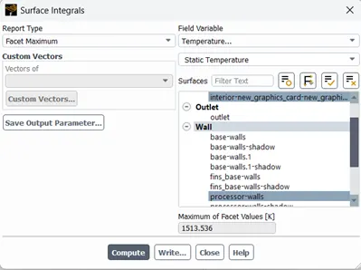
The maximum heat transfer coefficient was computed to be 1147.1625 Wm^-2K^-1.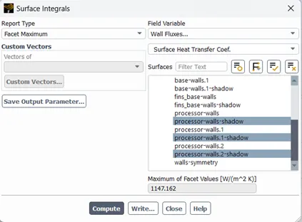
Post processed results:
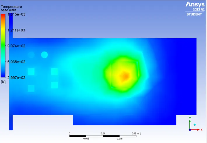
(Temperature plots for the base, the hot-spots near the area in contact with the processor is clearly visible.)
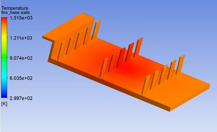
(Temperature plots for the fins. As aluminium is more conducting than the epoxy material of the base, the temperature distribution is more even. However, the area in contact with the processor is a clear hot-spot.)
It is clear from the post processed results that a more refined mesh will yield sharper plots for the temperature distribution across the components.Mesh refinement:
Body sizing methods were inserted for each of these components.
For Enclosure: the element length was set to 3mm.
For Base/Fins: the element length was set to 1mm.
For Processor: the element length was set to 0.5mm.

(Mesh statistics.)
The number of elements increased sizeably.
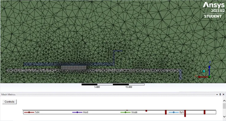
(The finer mesh.)
Solver set up remains unchanged exept for the velocity inlet speeds.
For inlet velocity as 1m/s:
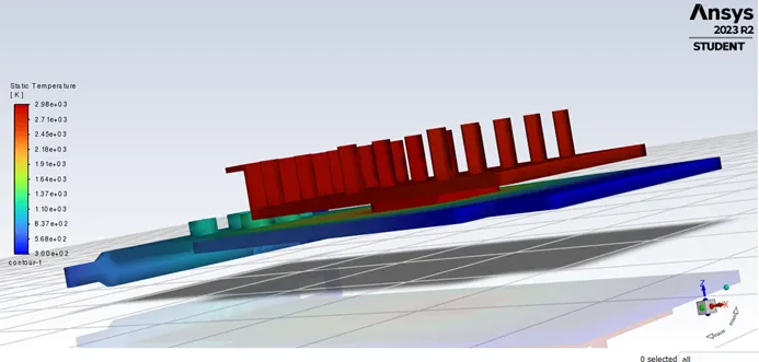
(Temperature contour.)
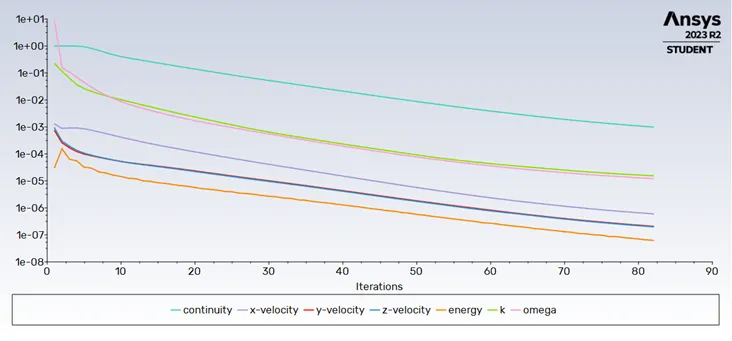
(Scaled Residuals.)
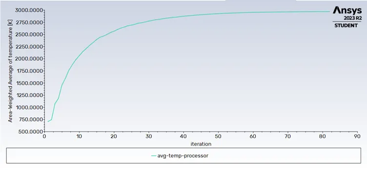
(Area-weighted average of surface temperature of the processor.)
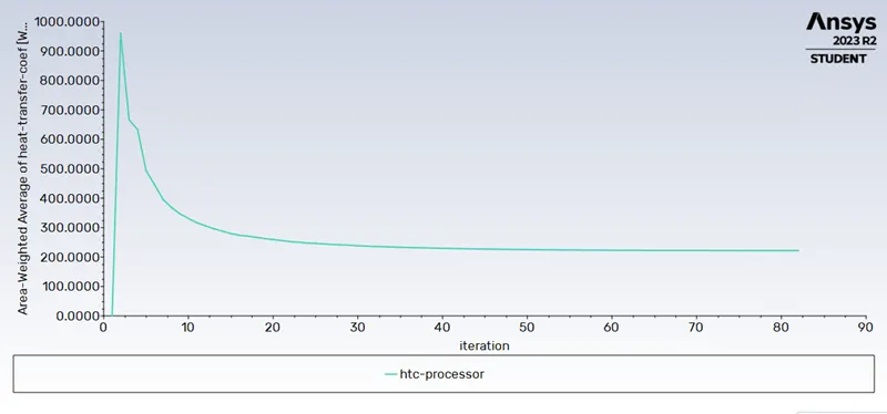
(Area weighted average of heat transfer coefficient of the processor.)
Computed value of the heat transfer coefficient (area weighted average) was 221.66599Wm^-2K^-1.
Computed value of the surface temperature (area weighted average) was 2970.0768K.
The maximum temperature on/in the processor was computed to be 2983.4316K.
The maximum heat transfer coefficient was computed to be 1357.6519Wm^-2K^-1.
Post processed results:
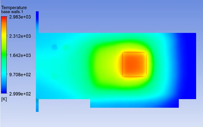
(The contours are much smoother and more refined.)
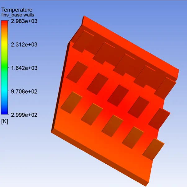
For inlet velocity as 3m/s:
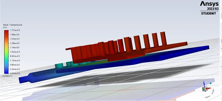
(Temperature contours.)
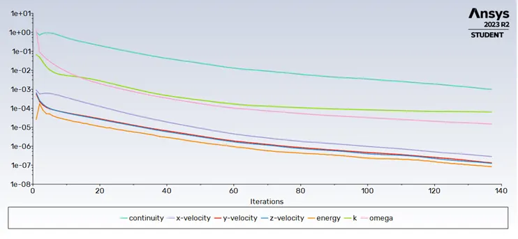
(Scaled residuals.)
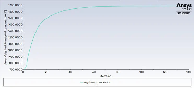
(Area-weighted average of surface temperature of the processor.)
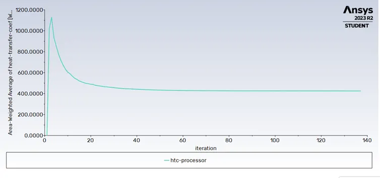
(Area weigthed average of heat transfer coefficient.)
Computed value of the heat transfer coefficient (area weighted average) was 425.50343Wm^-2K^-1.
Computed value of the surface temperature (area weighted average) was 1687.0669K.
The maximum temperature on/in the processor was computed to be 1700.0446K.
The maximum heat transfer coefficient was computed to be 2631.9241Wm^-2K^-1.
Post processed results:
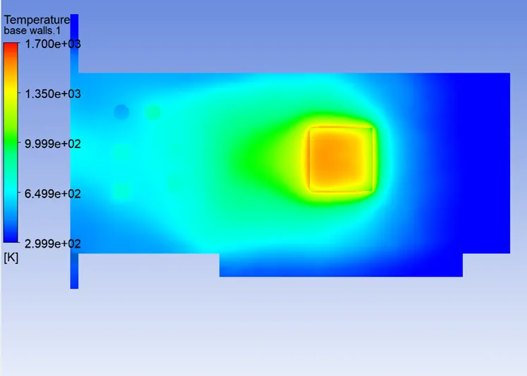
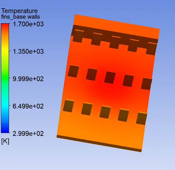
For inlet velocity as 3m/s:
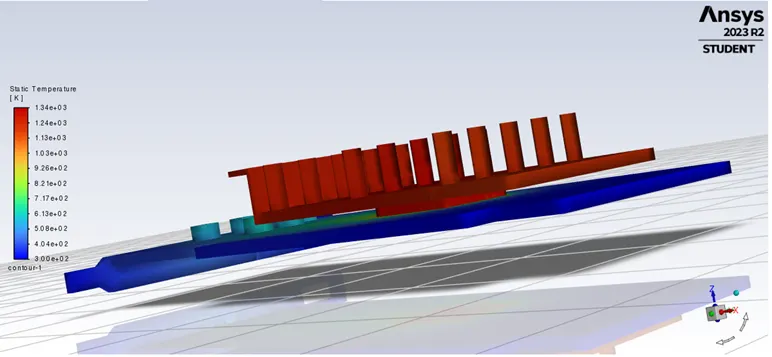 (Temperature contour.)
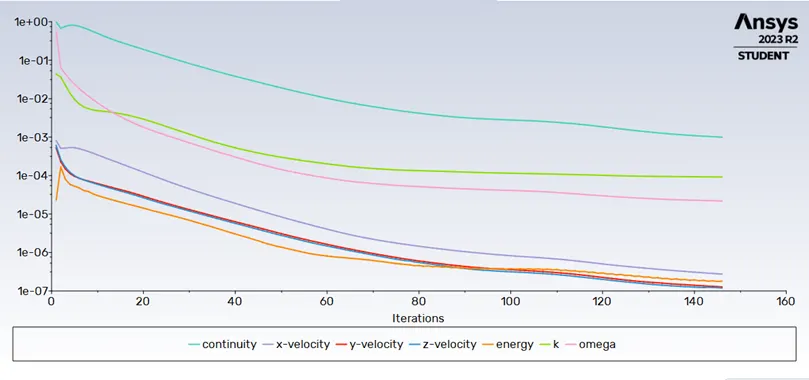 (Scaled residuals.)
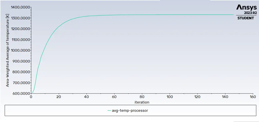
(Area-weighted average of surface temperature of the processor.)
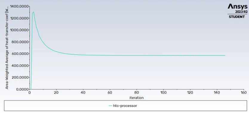
(Area weighted average of heat transfer coefficient of the processor.)
Computed value of the heat transfer coefficient (area weighted average) was 571.62667Wm^-2K^-1.
Computed value of the surface temperature (area weighted average) was 1330.2958K.
The maximum temperature on/in the processor was computed to be 1342.8597K.
The maximum heat transfer coefficient was computed to be 3524.5154Wm^-2K^-1.
Post-processed results:
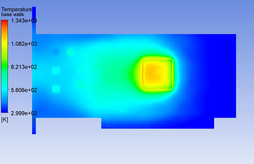
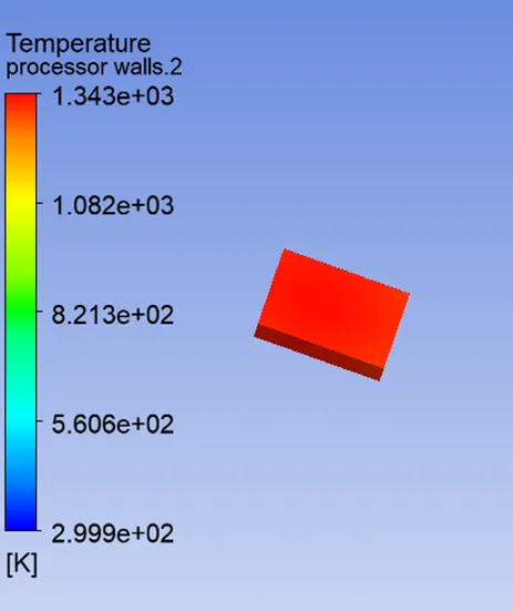
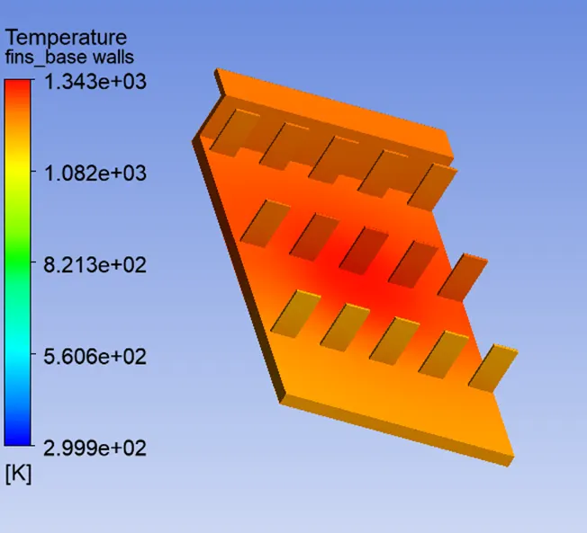
From the scaled residuals of all the cases, we can conclude that the results converge. Also, on observing the animations, after 110 iterations or so the contours seem to change very little, affirming that the results are convergent.
Observations and Conclusions
The data is summarised below in the form of a table:

As the inlet velocity increases, the heat transfer coefficient increases and consequently the processor temperatures show a decrease.
Thus, we can conclude that a higher inlet speed translates to better heat dissipation.
Hot spots next to the processor for all three cases:
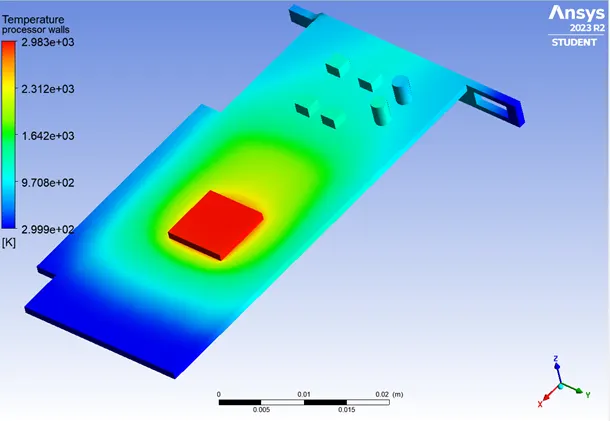
(For inlet velocity as 1m/s.)
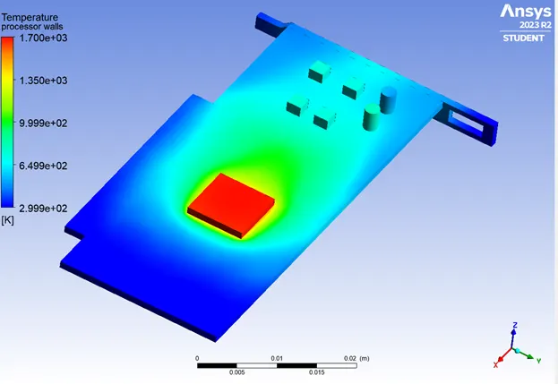
(For inlet velocity as 3m/s.)
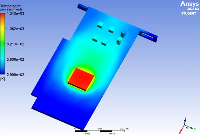
(For inlet velocity as 5m/s.)