Week 7 Challenge

# AIM

Load the vehicle parameters. Complete the vehicle model by modeling the remaining equations. Set simulation stop time to 598 sec.

The output should be the vehicle velocity.

# OBJECTIVE

To create a Simulink model of simple vehicle dynamics by using force equations acting on the vehicle with respect to the traction force taken as input and output to see its changes in the velocity of the vehicle.

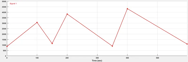
Inputs as traction force- From a signal builder block loaded with the traction force.

Output as Velocity of vehicle- To get by integrating the acceleration, which can be found from the actual traction force by dividing actual traction force by vehicle mass.

# THEORY

Forces acting on a vehicle:

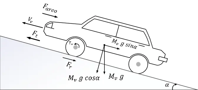
To make a vehicle move from rest positions a resultant force is needed. This resultant force is also known as traction force. This traction force is provided by the power train of a vehicle. But while the vehicle starts moving it gets opposed by some resistance forces.

These resistance forces are as shown in the above image and mentioned below as,

• Rolling resistance force(Fr).
• Aero dynamic force(Faero).
• Hill climbing force(Fhc) according to road grade ability.

Thus to overcome these resistance forces an additional traction force should be provided. The resultant traction force can be given as,

Force(Resultant)=Traction force -(Addition of above-mentioned resistance forces).

# SIMULINK MODEL

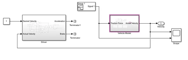
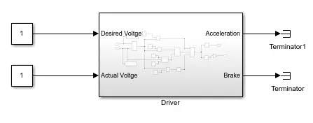
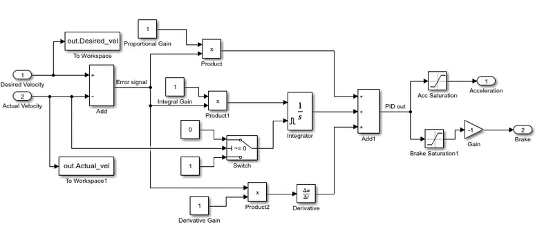
* Driver

* Vehicle Model

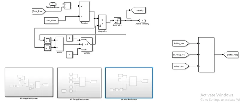
• Initially, the traction force is given from a signal builder block.

• All the resistance forces from subsystems are added by a sum block and given to a Goto block as Total_force. This added force is the total resistance force.
• This Total resistance force is subtracted from the Traction force input from the signal builder to get the resultant traction force.
• The resultant force is divided by mass to get the acceleration values.
• These acceleration values are integrated by using an integrator block to get the vehicle velocity output.
• The output from the integrator block is given to a saturation block to consider the velocity values from 0 to infinity as vehicle velocity output.
• The integrator block is get reset when the vehicle velocity reaches 0. This is done because as we are using integrator block it produces an integral windup.
• Integral windup means when the actual velocity tends to make a match with desired velocity,some times a shoot up of corrected signal occurs which again makes the next shootdown signal to attain its steady state desired velocity.
• To avoid this situation when the vehicle velocity gets to zero, the integrator block should get reseted.
• This makes the integrator start the action again from the initial state after the vehicle move from its rest condition.
• This action will avoid wind-up situations.
• This can be achieved in the model by verifying acceleration and velocity signals as reaching to Zero velocity.
• When the acceleration signal crosses 0 means the output from the memory block is 0,as the memory block output is precious input. Its makes a step delay.
• As the same for velocity signal crosses 0 means the output from memory block becomes 0.
• Both values are summed up and given to a switch condition.
• If summed up values is above 0, satisfying the switch condition. This makes no resetting of integrator for positive values.
• If the summed-up value gets 0, the switch condition fails. This makes the integrator reset.

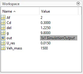
The assigned values are,

• Vehicle Mass: veh_mass =1500Kg.
• Acceleration due to gravity: g=9.8 m/s^2.
• Vehicle frontal area: Af=2 m^2.
• Aero drag coefficient: Cd=0.3
• Air density: del=1.225 Kg/m^3.
• Rolling resistance Coefficient: U_res=0.015.

The values assigned for model from variables are loaded from a .mat file as seen in the base workspace

* Construction of resistance forces subsystems :

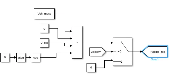
Rolling resistance force-

To find the rolling resistant force we have multiplied vehicle mass(Kg), acceleration due to gravity(m/S2), rolling resistance coefficient, and cosine of the angle of gradeability(in radian).

Frr=veh_mass*g*U_res*cos(0)

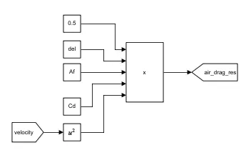
Aero drag resistance force:

To find the aero drag resistance force we have to multiply vehicle frontal area(m2), Air drag coefficient, air density(Kg/m3) and square of vehicle velocity(m/s).

Faero=0.5*Af*Cd*del*( velocity ^2)

The velocity of the vehicle is get from a From block(output of model) and squared by a square block.All these parameters are get multiplied to get the output as an aero drag resistance force.

Hill climbing resistance force:

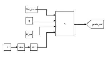
Hill climbing resistance force can be obtained by multiplying the Mass of the vehicle(Kg), Acceleration due to gravity(m/s^2), and sine of the angle of gradeability(in rad).

This can be given in relation as,

Fhc=veh_mass*g*sin(0)

All parameters are get multiplied in a product block and get hill climbing resistance force as shown below,

# SIMULATION RESULT

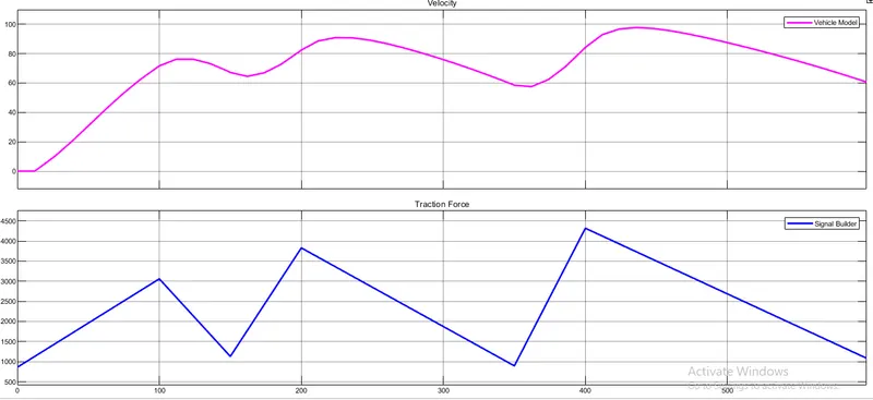
• Run the simulation for 598 secs and the vehicle velocity output as shown for the assigned vehicle parameter values
• The first plot shows the vehicle velocity output as per the input traction force given.
• The second plot shows the input traction force.
• From the scope we can clearly understand that, the vehicle velocity increase when input traction force increases, and velocity decrease when traction force decreases.
• Also at the initial starting duration of some time vehicle velocity is in zero although the traction force is around 900 N.
• This occurs as the resistance force is higher than the initial starting traction force.

# CONCLUSION

Completed the vehicle model by modeling the remaining equations.