Project

# AIM

To prepare a technical report on the Simulation of BAJA All-Terrain Vehicle (ATV) under different conditions.

# OBJECTIVE

Carry out a system-level simulation of an all-terrain vehicle and prepare a technical report explaining the model properties & comments on the results.

# THEORY

* All-Terrain Vehicle

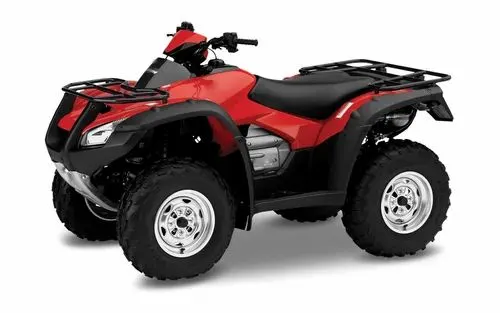
Fig 1: All-Terrain Vehicle

An all-terrain vehicle (ATV) is defined as a motorized off-highway vehicle designed to travel on four low-pressure or non-pneumatic tires, having a seat designed to be straddled by the operator and handlebars for steering control. ATVs have many purposes such as joy riding, adventure sports, convenience farming, and border security. Their trails are not commonplace, many riders use them on hilly tracks, sand dunes, forest areas, and another terrain that is not accessible by street vehicles.

* Basic Automatic Transmission

The gears are literally gears-- interlocking, toothed wheels that help to transmit and modify rotary motion and torque. A combination of planetary gears creates all of the different gear ratios that the transmission can produce, typically four forward gears and one reverse gear. When this type of transmission cycles through its gears, the driver can feel jolts as each gear is engaged.

* Continuously Variable Transmission (CVT) Vehicle

Continuously Variable Transmission (CVT) does not make use of gears like a basic automatic transmission. Rather, it uses 2 pulleys linked by a belt. It’s like a snowmobile transmission: One pulley connects to the engine and the other one links to the transmission. The belt transfers the power between them. Depending on the vehicle and the driver, CVT can provide a smoother driving experience when comparing it to a traditional automatic. According to Carfax, one of the most significant advantages of having a CVT is that they are often more fuel-efficient than a regular automatic.

Fig 2: Continuously Variable Transmission (CVT)

Working Principle

The variable-diameter pulleys are the heart of CVT. Each pulley is made of two 20-degree cones facing each other. A belt rides in the groove between the two cones. The V-belts are preferred if the belt is made of rubber. V-belts get their name from the fact that the belts bear a V-shaped cross-section, which increases the frictional grip of the belt. When two cones of the pulley are far apart (when the diameter increases), belt rides lower in the groove, and the radius of the belt loop going around the pulley gets smaller. When the cones are close together (when the diameter decreases), belt rides higher in the groove, and the radius of the belt loop going around the pulley gets larger. CVTs may use hydraulic pressure, centrifugal force or spring tension to create the force necessary to adjust the pulley halves.

Variable-diameter pulleys always come in pairs. One of the pulleys, known as the drive pulley (or driving pulley), is connected to the crankshaft of the engine. The driving pulley is called the input pulley because it's where the energy from the engine enters the transmission. The second pulley is called the driven pulley because the first pulley is turning it. As an output pulley, the driven pulley transfers energy to the driveshaft.

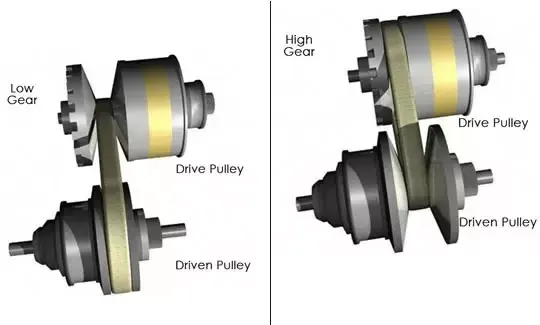
Fig 3: Pulleys based on CVT

When one pulley increases its radius, the other decreases its radius to keep the belt tight. As the two pulleys change their radius relative to one another, they create an infinite number of gear ratios -- from low to high and everything in between. For example, when pitch radius is small on the driving pulley and large on the driven pulley, then the rotational speed of the driven pulley decreases, resulting in the lower “gear.” When the pitch radius is large on the driving pulley and small on the driven pulley, then the rotational speed of the driven pulley increases, resulting in higher “gear.” Thus, a CVT has an infinite number of "gears" that it can run through at any time, at any engine or vehicle speed.

# SIMULINK MODEL 0F BAJA ATV

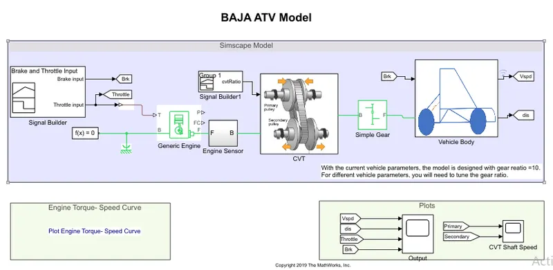
Fig 4: Model of BAJA ATV

* Continuously Variable Transmission (CVT) Drive

It is better to have more gears in transmission since it can optimize engine speed in a variety of driving conditions. That means low gears can provide better acceleration while higher gears can maximize fuel economy. CVTs differ from traditional automatic transmissions in that they don't have gears that provide "steps" between low- and high-speed operations. Instead, the majority of them work via a pair of variable diameter, cone-shaped pulleys connected by a steel or composite belt. The halves of each pulley are aligned with pointed ends of the cones touching. These form a V-shaped groove in which the connecting belt rides. One side of the pulley is fixed, and other side is movable, actuated by a hydraulic cylinder. The cylinder can increase or decrease the amount of space between the two sides of the pulley. This allows the belt to ride lower or higher along the walls of the pulley, depending on driving conditions. thereby changing the "gear" ratio.

* CVT Block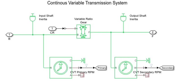

Fig 5: CVT Block

Represents a variable ratio gearbox such as implemented by mechanical belt CVT, electric, or hydraulic transmissions. physical signal input r defines a ratio of input to the output angular shaft velocities. Connections B (base) and F (follower) are mechanical rotational conserving ports. Specify the relation between base and follower rotation directions with the Output shaft rotates parameter.

In CVT the variable diameter pulleys play a major role. One is the driver and the other is the driven pulley, they come in pairs and are connected to the crankshaft of the engine. when the pitch radius is small on the driving pulley and large on the driven pulley, then the rotational speed of the driven pulley decreases, resulting in the lower “gear.” When the pitch radius is large on the driving pulley and small on the driven pulley, then the rotational speed of the driven pulley increases, resulting in a higher gear. Thus, a CVT has an infinite number of gears that it can run through at any time, at any engine or vehicle speed.

* Generic Engine

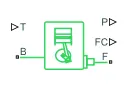
Fig 6: Generic Engine

Represents a system-level model of spark-ignition and diesel engines suitable for use at the initial stages of modeling when only the basic parameters are available. Optional idle speed and red line are included. The throttle input signal T lies between zero and one and specifies the torque demanded from the engine as a fraction of the maximum possible torque. Connections F and B are mechanical rotational conserving ports associated with the engine crankshaft and engine block. Connections P and FC are physical signal output ports through which engine power and fuel consumption rate are reported.

* Simple Gear

The simple gear is a combination of a driver and driven gear where the speed is reduced by the gear ratio. The simple gear block is nothing but the fixed-ratio gear or gearbox, where follower to base teeth ratio is set as 12.

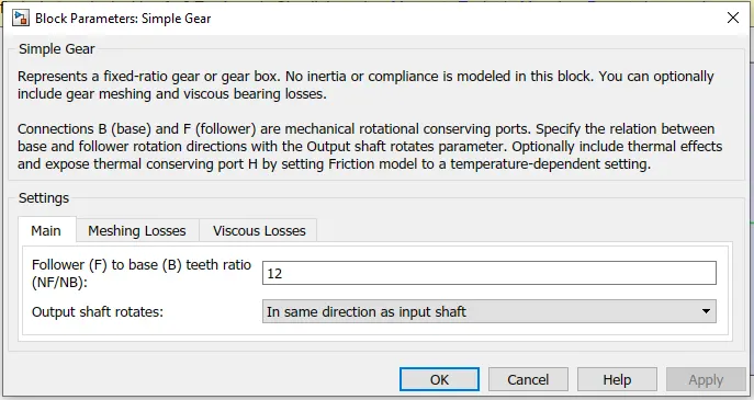
Fig 7: Simple Gear Block

* Vehicle Body

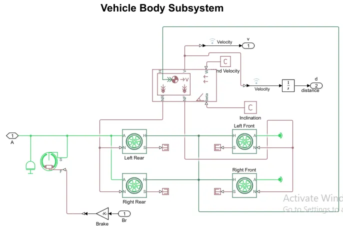
Fig 8: Vehicle Body

The Vehicle subsystem accounts for the forces acting on the body. For a vehicle to be mobile, it has to produce tractive effort to overcome forces due to drag, rolling resistance, hill climb, and also acceleration. In the subsystem, a double shoe brake is applied to the rear wheels. Two of these are kept at both ends to prevent the action of unbalanced forces. The parameters for the vehicle are given below.

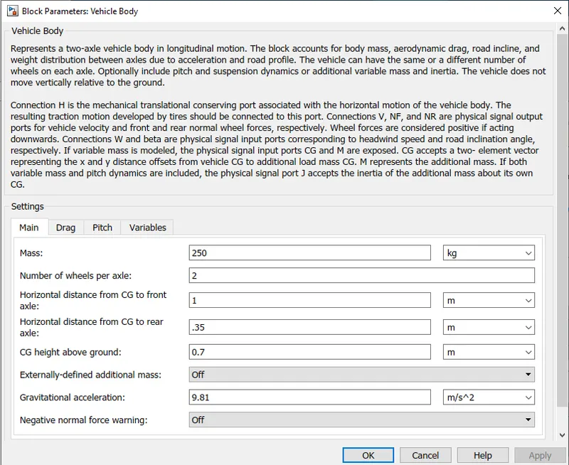
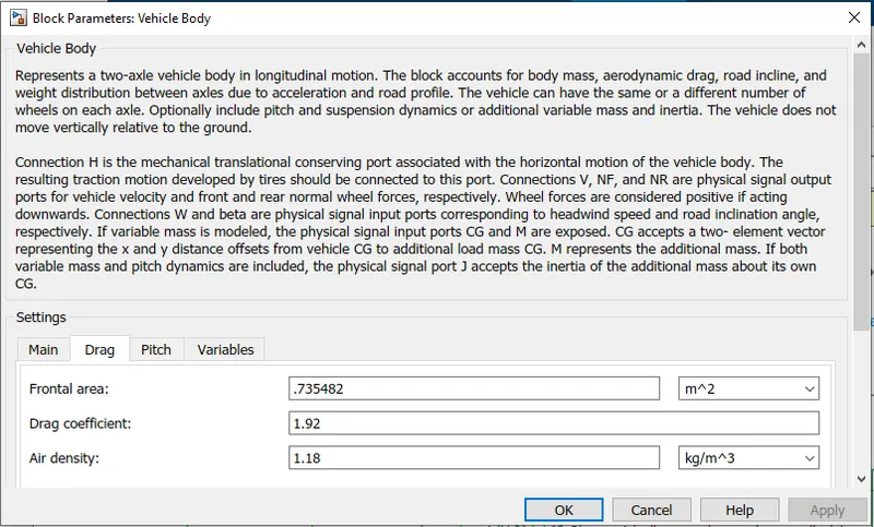
Fig 9: Parameters of Vehicle Body

# CASE STUDY

* Case 1: Simulation of BAJA ATV model with CVT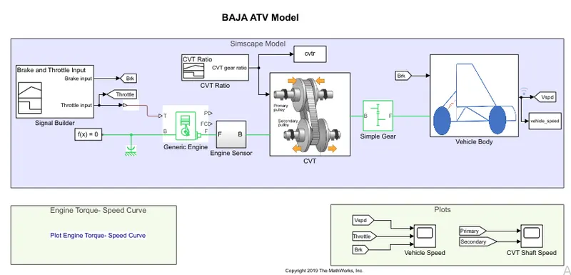

Fig 10: Simulation of BAJA ATV model with CVT

* Brake and Throttle input

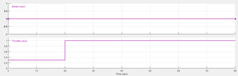
Fig 11: Brake and Throttle input

• The throttle signal is generated by the signal builder and inputted to the generic engine.
• Brake input is constant, zero throughout the time 80s.
• Throttle input is .3 for the first 20s, accelerates to 1 at the same and remains constant throughout the remaining till 80s.

* CVT Gear Ratio

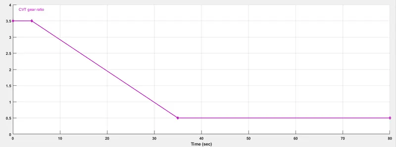
Fig 12: CVT Gear Ratio

• The gear ratio is provided to the CVT through Signal Builder.
• The gear ratio is 3.5 for the first 4s.
• Then drop down to 0.5 till 35s and remains constant thereafter till the 80s.

* Output Waveforms

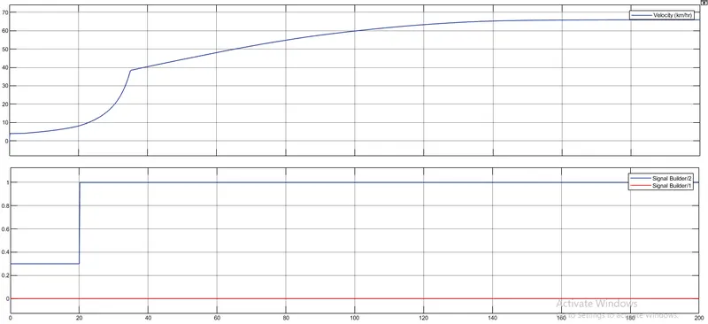
Fig 13: Velocity Of the Vehicle

• From the graph, we can infer that when the brake is not applied during the drive cycle and the throttle is constant till the 20s and being increased from 0.3 to 1 from the 20s, where it remains constant for the rest of the run.
• With the increase in throttle, the vehicle speed also get increases.
• From the above plot, the vehicle accelerated from 0 to 38kmph very gradually and after attaining a velocity of 65kmph it remains constant throughout the cycle.

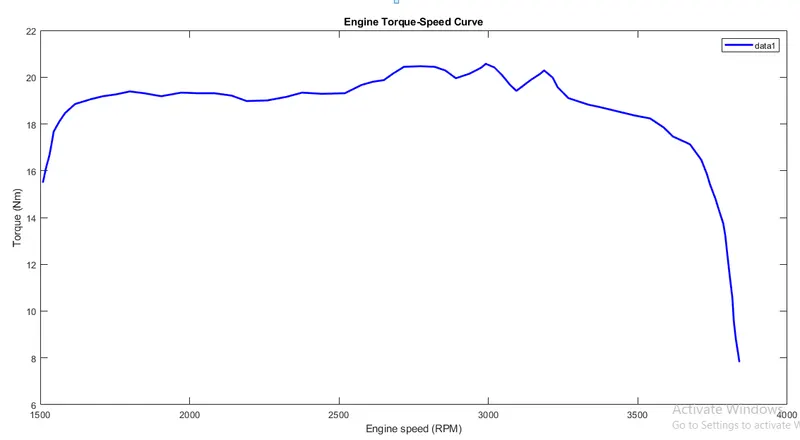
Fig 14: Torque Speed Curve

• The Torque and Speed are inputted from the MATLAB Workshop window to the generic engine block to generate the output rpm accordingly.
• This plot is common for all cases because it's a default input to the engine.

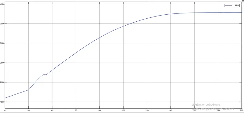
Fig 15: Engine Speed

• Here we can see the engine rpm generated accordingly w.r.t to the throttle, speed, and torque inputs.

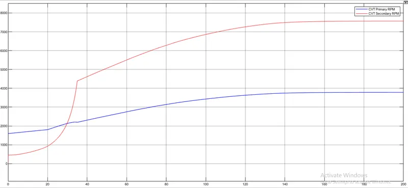
Fig 16: CVT Shaft Speed

• The speed of the driving and driven shaft depending on the gear ratios.
• There is a steady increase in CVT secondary rpm up to gear ratio 0.5, after that it gradually increased
• This increase and decrease in the rpm values of primary and secondary pulleys depend on the throttle values and gear ratios.

* Case 2: Simulation of bAJA ATV model with CVT and Dashboard

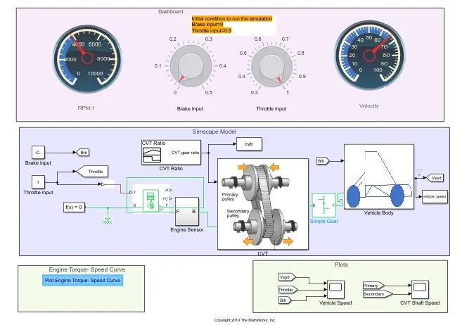
Fig 17: Simulation of bAJA ATV model with CVT and Dashboard

• Here input values of the throttle and brake input are not given through signal builders
• Throttle input and Brake input are connected to the dashboard, here the display of RPM and Velocity can be seen during the change in throttle and brake values.
• The initial condition is 0 brake and 0.3 throttle value.

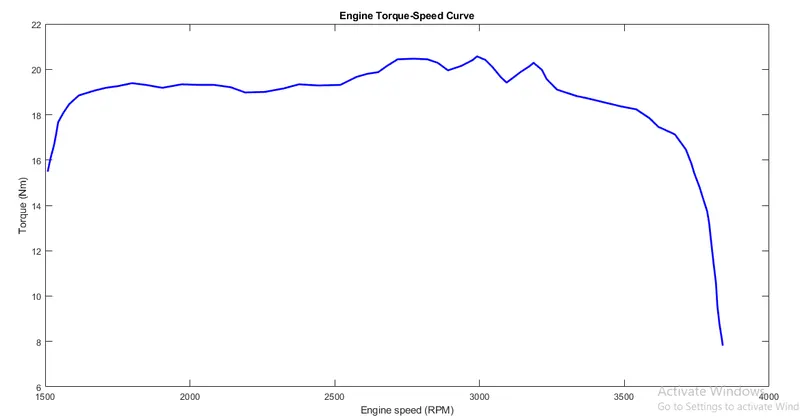
Fig 18: Torque Speed Curve

• The Torque and Speed are inputted from the MATLAB Workshop window to the generic engine block to generate the output rpm accordingly.
• This plot is common for all cases because it's a default input to the engine.

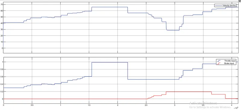Fig 19: Velocity Of the Vehicle

• The Velocity of the vehicle increases with an increase in throttle input.
• Velocity decreases with an increase in the brake input.
• In the graph Increase and decrease of velocity are shown in different Throttle and Brake values.

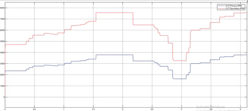
Fig 20: CVT Shaft Speed

• The speed of the driving and driven shaft depending on the gear ratios.
• The variation in the speed of the primary and secondary pulley depends on the throttle and brake values.
• As the throttle value increases, the rpm of the two pulleys also increases.
• As the brake Value increases, the rpm of the two pulleys decreases.
• From the graph, the rpm value of the secondary pulley is more than the primary pulley, so the radius of the secondary pulley is smaller than the primary pulley.

* Case 3: Simulation of BAJA ATV model with a Lookup table

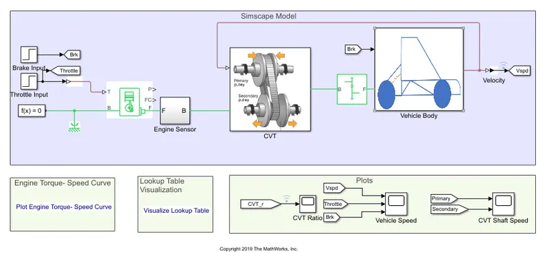
Fig 21: Simulation of bAJA ATV model with a Lookup table

• The only difference between this model and the first model is that in this model gear ratio input to CVT is provided using a lookup table.

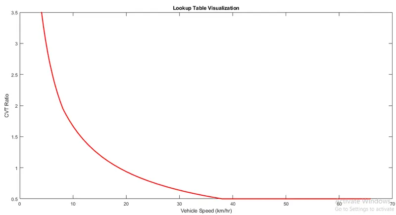
Fig 22: Lookup Table

• The graph is a testament to the fact that at high speed the CVT Ratio decreases.
• it is closed-loop feedback, according to the velocity the CVT ratios are given.

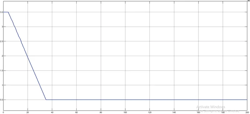
Fig 23:CVT gear Ratio

*Output Waveforms

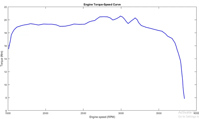
Fig 24: Torque Speed Curve

• The Torque and Speed are inputted from the MATLAB Workshop window to the generic engine block to generate the output rpm accordingly.
• This plot is common for all cases because it's a default input to the engine.

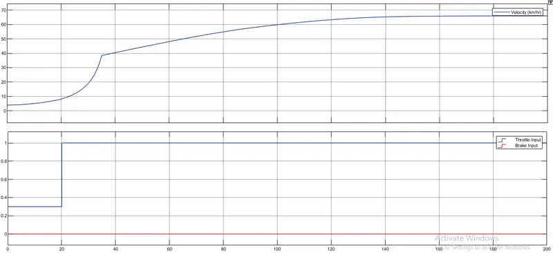
Fig 25: Velocity Of the Vehicle

• From the graph, we can infer that when the brake is not applied during the drive cycle and the throttle is constant till the 20s and being increased from 0.3 to 1 from the 20s, where it remains constant for the rest of the run.
• With the increase in throttle, the vehicle speed also get increases.
• From the above plot, the vehicle accelerated from 0 to 38kmph very gradually and after attaining a velocity of 65kmph it remains constant throughout the cycle.

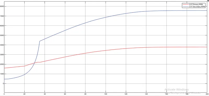
Fig 26: CVT Shaft Speeds

• The speed of the driving and driven shaft depending on the gear ratios.
• This increase and decrease in the rpm values of primary and secondary pulleys depend on the throttle values and gear ratios.

* Case 4: Simulation of BAJA ATV model with a Lookup table and Dashboard

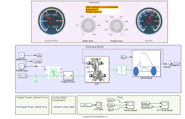
Fig 27: Simulation of bAJA ATV model with a Lookup table and Dashboard

• Throttle input and Brake input are connected to the dashboard, here the display of RPM and Velocity can be seen during the change in throttle and brake values.
• The initial condition is 0 brake and 0.3 throttle value.
• In the above model, Lookup table data has been assigned as input to the CVT instead of CVT ratios.
• The lookup table is created by a program in MATLAB and data has been assigned as an input to the CVT.

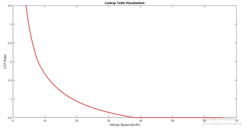
Fig 28: Lookup Table

• The graph is a testament to the fact that at high speed the CVT Ratio decreases.
• it is closed-loop feedback, according to the velocity the CVT ratios are given.

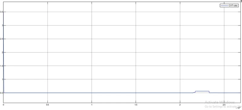
Fig 29: Gear Ratio

* Output Waveforms

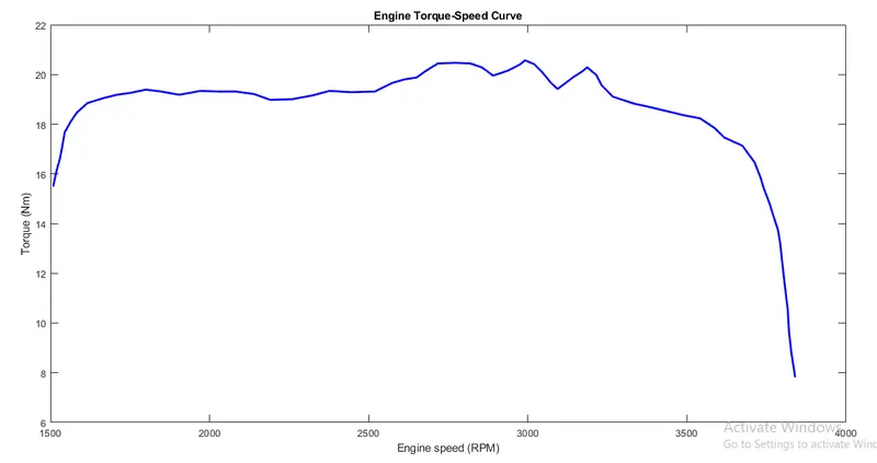
Fig 30: Torque Speed Curve

• The Torque and Speed are inputted from the MATLAB Workshop window to the generic engine block to generate the output rpm accordingly.
• This plot is common for all cases because it's a default input to the engine.

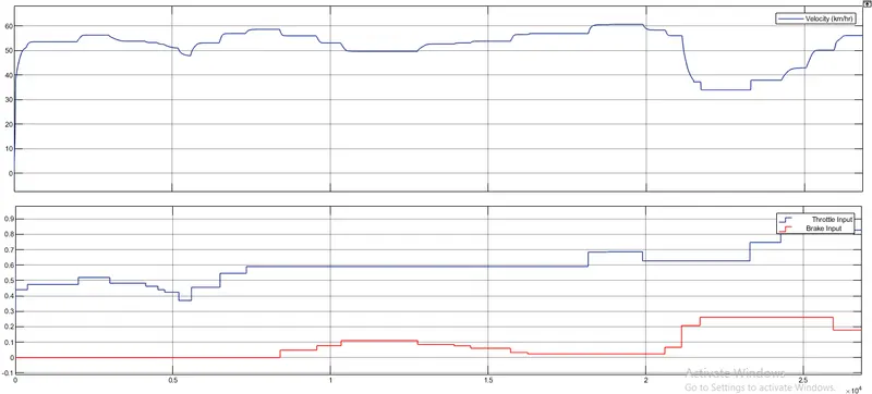
Fig 31: velocity Of the Vehicle

• The Velocity of the vehicle increases with an increase in throttle input.
• Velocity decreases with an increase in the brake input.
• In the graph Increase and decrease of velocity are shown in different Throttle and Brake values.

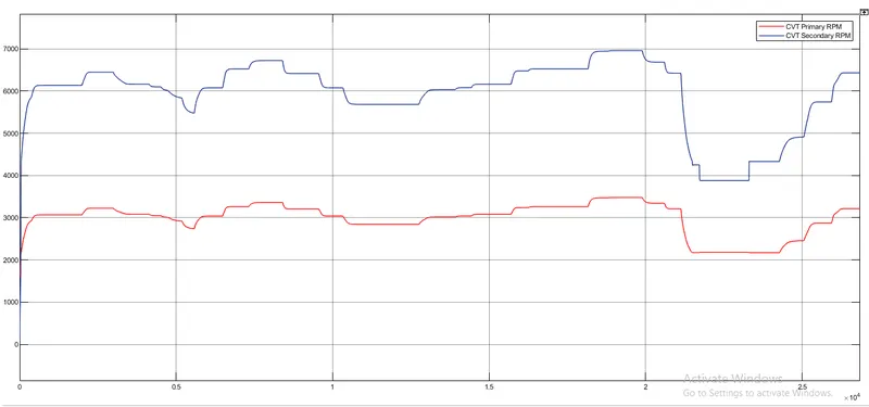
Fig 32: CVT Shaft Speeds

• The speed of the driving and driven shaft depending on the gear ratios.
• The variation in the speed of the primary and secondary pulley depends on the throttle and brake values.
• As the throttle value increases, the rpm of the two pulleys also increases.
• As the brake Value increases, the rpm of the two pulleys decreases.
• From the graph, the rpm value of the secondary pulley is more than the primary pulley, so the radius of the secondary pulley is smaller than the primary pulley.

# CONCLUSION

Hence the given BAJA ATV Model was simulated successfully and from the above results, we can infer that: Velocity, CVT shaft speed, and Engine Speed are directly proportional to the throttle input and inversely proportional to the brake input.CVT ratios are directly proportional to Torque and inversely proportional to the throttle input.CVT secondary pulley rpm is more than primary because it depends on the gear ratio.