Challenge

Week 7 Challenge

SShriraam S19 Apr 2025

MATLAB

Below are the vehicle parameters considered for this vehicle model:

m = 1200; % mass [kg]

g = 9.81; % gravity [m/s^2]

Cr = 0.015; % rolling resistance coefficient

rho = 1.225; % air density [kg/m^3]

Cd = 0.32; % drag coefficient

A = 2.2; % frontal area [m^2]

slope_deg = 5; % slope in degrees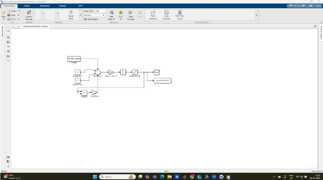

VehicleDynamicsModel_Enhanced.slx

This model simulates the longitudinal dynamics of a vehicle, incorporating various real-world physical effects. Let’s break it down component by component:

Main Subsystems & Blocks

Block	Description
Throttle Input (Time-Varying)	Implements a step-based or custom function input to simulate gas pedal application over time.
Vehicle Mass(1/m)	Implements Newton's 2nd Law $a = \frac{F}{m}$ a=mF, used after summing all the forces.
Sum of Forces Block	Adds up all the forces: +Throttle Force, -Rolling Resistance, -Gravity Component, -Aerodynamic Drag.
Integrator	Integrates acceleration to compute velocity over time. Output = vehicle velocity.
Scope	Displays the velocity vs time. What you shared previously.
To Workspace	Exports velocity to MATLAB for plotting or analysis.

Force Components Modeled

Force	Formula	Block Function
Throttle Force	$F_{throttle} = Throttle Input \times Max Force$ Fthrottle=Throttle Input×Max Force	Derived from the input block
Rolling Resistance	$F_{r} = C_{r} \cdot m \cdot g$ Fr=Cr⋅m⋅g	Resists motion due to tires
Gravity (Slope)	$F_{g} = m \cdot g \cdot \sin (θ)$ Fg=m⋅g⋅sin(θ)	Component of gravity on an incline
Aerodynamic Drag	$F_{d} = 0.5 \cdot ρ \cdot C_{d} \cdot A \cdot v^{2}$ Fd=0.5⋅ρ⋅Cd⋅A⋅v2	Increases with velocity squared

Simulation Behavior Based on the Model

0–100 sec: Vehicle is idle (no throttle).
100–130 sec: Throttle is applied → acceleration.
130–500 sec: Vehicle reaches and maintains cruise speed.
After 500 sec: Throttle removed → resistance forces slow vehicle.

Outputs
- Scope: Visualizes vehicle velocity.
- To Workspace Block: Sends velocity to MATLAB variable (vehicle_velocity)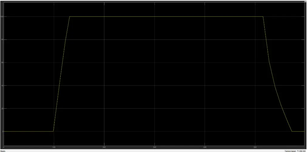
  
  Understanding the vehicle velocity over time:
  
  Interpreting the Plot
  Time Axis (X-axis)
  - The horizontal axis runs from 0 to 598 seconds.
  - This aligns with your simulation stop time of 598 sec.
  Velocity Axis (Y-axis)
  - The vertical axis shows velocity, in what appears to be km/h or m/s (depending on your units in Simulink).
  - Values range from 0 up to ~100, then back down.
  Phases of the Simulation
  0–100 seconds:
  - Velocity remains at 0
  - No throttle or driving force applied. Vehicle is stationary.
  100–130 seconds:
  - Sharp acceleration
  - Throttle input kicks in (based on time-varying input).
  - Vehicle gains speed rapidly.
  130–500 seconds:
  - Steady high-speed cruising
  - Velocity plateaus around 100 units.
  - Net forces likely balance (engine force ≈ total resistive forces).
  - Vehicle moves at constant speed.
  500–598 seconds:
  - Deceleration phase
  - Likely the throttle input drops to zero or is reduced significantly.
  - Resistance forces (like drag, gravity on slope, rolling resistance) dominate.
  - Vehicle slows down and comes to a stop by ~598 sec.
  Real-World Interpretation
  This simulation mimics a typical driving scenario:
  1. Vehicle waits initially,
  2. Accelerates to cruising speed,
  3. Maintains that speed for some time,
  4. Then decelerates and stops.
  This behavior is likely driven by your time-varying throttle input combined with:
  - Rolling resistance
  - Aerodynamic drag
  - Gravity due to road slope

Week 7 Challenge

Main Subsystems & Blocks

Force Components Modeled

Simulation Behavior Based on the Model

Outputs

Interpreting the Plot

Time Axis (X-axis)

Velocity Axis (Y-axis)

Phases of the Simulation

0–100 seconds:

100–130 seconds:

130–500 seconds:

500–598 seconds:

Real-World Interpretation

Ship work like this
in your own course.

Talk to a career counsellor

Main Subsystems & Blocks

Force Components Modeled

Simulation Behavior Based on the Model

Outputs

Interpreting the Plot

Time Axis (X-axis)

Velocity Axis (Y-axis)

Phases of the Simulation

0–100 seconds:

100–130 seconds:

130–500 seconds:

500–598 seconds:

Real-World Interpretation

Ship work like thisin your own course.

Talk to a career counsellor

Ship work like this
in your own course.