Week 7 - Auto ignition using Cantera

 Aim:-

To find the autoignition time of methane under varying conditions of pressure & temperature and analyze the evolution of molar concentrations of reactants with combustion progress.

For this, we will consider:

Case -1: Auto-ignition time with

A. Constant temperature of 1250 K and pressure variation from 1 to 5 atmospheres.

B. Constant pressure of 5 atmospheres and temperature variation from 950 K to 1450 K.

Case- 2: Molar concentrations at

A.1000 K and 5 atm.

B.500 K and 5 atm.

Introduction:-

The lowest temperature at which ignition starts is the Auto-ignition temperature. This temperature can vary based on the initial temperature, pressure, and element concentrations. There is also time associated with autoignition which is called Ignition delay. Once the fuel and air mixture are together, after a certain time the ignition begins, and this time gap is referred to as ignition delay. Fuels are characterized by ignition delay.

The lower the initial temperature, the higher will be the ignition delay. But this is not always true. There is a term called Negative temperature co-efficient regime, which indicates the region on the ignition time vs temperature. In this region, as the initial or ignition temperature increases, the ignition delay increases for some time before dipping. This is also a fuel property, which means it varies for different fuels. 

Practically there are experiments utilized to estimate ignition delay such as - the shocktube experiment and rapid combustion experiment. In terms of equations, to determine ignition delay, only species and energy equations have to be solved - through these equations, the rate of temperature rise can be calculated. So, when ignition starts, the temperature hikes very rapidly and attains the maximum value. Through this value, ignition delay can be calculated.

To satisfy the current aims, Cantera is used. In Cantera, different reactors can be used based on the problem requirement. Each reactor will have a certain volume and its governing equations. The details of governing equations are provided on the Cantera website. In a reactor, at a particular state, properties such as temperature and pressure remain constant.

Based on the reactor defined, a reactor network can be used, which integrates all different states of the reactor using advanced methods. The simulation presented here is the 0D simulation, as only the temporal evolution of the gas mixture towards equilibrium is considered.

Approach:-

Combustion will be simulated in python using the reactor network available in the Cantera package.  A Cantera reactor represents the simplest form of a chemically reacting system and has the following characteristics:

1. It is a thermodynamic control volume V, in which all state variables are homogeneously distributed.
2. The system is generally unsteady -- that is, all states are functions of time so that transient state changes due to chemical reactions are possible.
3. Thermodynamic (but not chemical) equilibrium is assumed to be present throughout the reactor at all instants of time.

The state of this reactor will be changed through a series of many equilibrium states each separated by a small time step so that the process (combustion) can be closely approximated as a quasi-static process.

Code:-

1. For simulating combustion, a function 'combust()' is defined which takes initial temperature, pressure, and species concentration as user inputs. Optionally, the time step size can be changed & also whether to simulate only till ignition.
2. Inside combust(), a reactor object is made that mimics an ideal gas combustion mixture at a given state.
3. Next, the reactor network object is made from the reactor object which will simulate the system.
4. A solution array is made using Cantera so that the state at each time step can be saved.
5. The time loop is then run. Each iteration changes time by a small amount then, the reactor state is computed at that time using state variables at the previous time step.
6. As soon as the reactor temperature increases above 400 K of initial value auto-ignition has occurred and the temperature is saved.
7. The gas object, states (Solution array), and ignition_delay are returned by the function.
8. The results are plotted after providing appropriate arguments to combust().

Program:-

import cantera as ct
import numpy as np
import matplotlib.pyplot as plt

def combust(T: float, P: float, spcies_dict: dict, reactor: str, dt: float= 0.0005, till_ignition: bool=True):
    gas = ct.Solution('gri30.yaml')
    gas.TPX = T, P, spcies_dict
    # Selecting reactor
    if reactor == 'constant temperature':
        r = ct.IdealGasReactor(gas)
    
    elif reactor == 'constant pressure':
        r = ct.IdealGasConstPressureReactor(gas)
    
    else:
        raise TypeError(f"Improper reactor type '{reactor}'")

    # Making reactor network
    sim = ct.ReactorNet([r])
    # Making a solution array  object
    states = ct.SolutionArray(gas, extra=['time_in_ms', 'time_in_sec'])

    # Simulates for  10 sec = dt*n_steps
    simulation_time = 10
    # time step is dt
    n_steps = int(simulation_time/dt)
    ignition_delay = 0.0
    
    # A flag so that auto-ignition temperature is computed only 
    # once, the first time temperatue spikes by 400 [K]
    ignited = False
    
    # Time loop
    time = 0.0
    for n in range(n_steps):
        time += dt
        sim.advance(time)
        states.append(r.thermo.state, time_in_sec= time, time_in_ms= time*1e3)
        
        if ignited == False:
            if states.T[n] >= (T + 400):
                ignition_delay = time
                ignited = True
                if till_ignition == True:
                    break

    return gas, states, ignition_delay

# %%
# PART I-A
fig1, axs = plt.subplots(2,1, figsize=(10, 10), layout='tight')

igd_lst = []
P = np.linspace(1,5,9)
for t in P:
    _, states, igd = combust(1250, t*ct.one_atm, {'CH4':1, 'O2':2, 'N2': 7.52}, 'constant temperature', dt= 2e-4)
    axs[0].plot(states.time_in_ms, states.T, '.-', label= f'{t: .3} atm, I.D. = {igd*1000: .5} ms')
    igd_lst.append(igd)

axs[0].set_xlabel('Time [ms]$\longrightarrow$')
axs[0].set_ylabel("Flame Temperature [K]$\longrightarrow$")
axs[0].grid(linestyle='-.')
axs[0].legend()

axs[1].plot(np.array(igd_lst)*1000, P, '.-')
axs[1].set_xlabel('Auto-ignition time [ms]$\longrightarrow$')
axs[1].set_ylabel("Pressure [atm]$\longrightarrow$")
axs[1].grid(linestyle='-.')

fig1.suptitle(f"Auto-ignition of methane at 1250 Kn and pressure variation")
# %%
# PART I-B
fig2, axs = plt.subplots(2,1, figsize=(10, 10), layout='tight')

igd_lst = []
T = np.linspace(950, 1450, 9)
for t in T:
    _, states, igd = combust(t, 5*ct.one_atm, {'CH4':1, 'O2':2, 'N2': 7.52}, 'constant pressure')
    axs[0].plot(states.time_in_ms, states.T, '.-', label= f'{t} K, I.D. = {igd*1000: .5} ms')
    igd_lst.append(igd)

axs[0].set_xlabel('Time [ms]$\longrightarrow$')
axs[0].set_ylabel("Flame Temperature [K]$\longrightarrow$")
axs[0].grid(linestyle='-.')
axs[0].legend()

axs[1].plot(np.array(igd_lst)*1000, T, '.-')
axs[1].set_xlabel('Auto-ignition time [ms]$\longrightarrow$')
axs[1].set_ylabel("Initial temperature [K]$\longrightarrow$")
axs[1].grid(linestyle='-.')

fig2.suptitle(f"Auto-ignition of methane at 5 atmn and initial temperature variation")
#%%
# PART II-A & B
gasA, statesA, igdA = combust(1000, 5*ct.one_atm, {'CH4':1, 'O2':2, 'N2': 7.52}, 'constant temperature', till_ignition= False)
gasB, statesB, igdB = combust(500, 5*ct.one_atm, {'CH4':1, 'O2':2, 'N2': 7.52}, 'constant temperature', dt= 0.01, till_ignition= False)
#%%
fig3, axs = plt.subplots(3,1, figsize=(10, 10), layout='tight')

axs[0].plot(statesA.time_in_sec, statesA.X[:,gasA.species_index('H2O')], '.-', color='red', label= f'1000 K, I.D. = {igdA*1000: .5} ms')
axs[0].plot(statesB.time_in_sec, statesB.X[:,gasB.species_index('H2O')], '.-', label= f'500 K, I.D. = {igdB*1000: .5} ms')
axs[0].set_ylabel("$[H_2O]$")
axs[0].grid(linestyle='-.')
axs[0].legend()

axs[1].plot(statesA.time_in_sec, statesA.X[:,gasA.species_index('O2')], '.-', color='red', label= f'1000 K, I.D. = {igdA*1000: .5} ms')
axs[1].plot(statesB.time_in_sec, statesB.X[:,gasB.species_index('O2')], '.-', label= f'500 K, I.D. = {igdB*1000: .5} ms')
axs[1].set_ylabel("$[O_2]$")
axs[1].grid(linestyle='-.')
axs[1].legend()

axs[2].plot(statesA.time_in_sec, statesA.X[:,gasA.species_index('Oh')], '.-', color='red', label= f'1000 K, I.D. = {igdA*1000: .5} ms')
axs[2].plot(statesB.time_in_sec, statesB.X[:,gasB.species_index('Oh')], '.-', label= f'500 K, I.D. = {igdB*1000: .5} ms')
axs[2].set_ylabel("$[OH]$")
axs[2].grid(linestyle='-.')
axs[2].legend()

fig3.supxlabel('Time [sec]$\longrightarrow$')
fig3.supylabel("Molar concentration$\longrightarrow$")

plt.show()

Results:- 

Case 1-A:

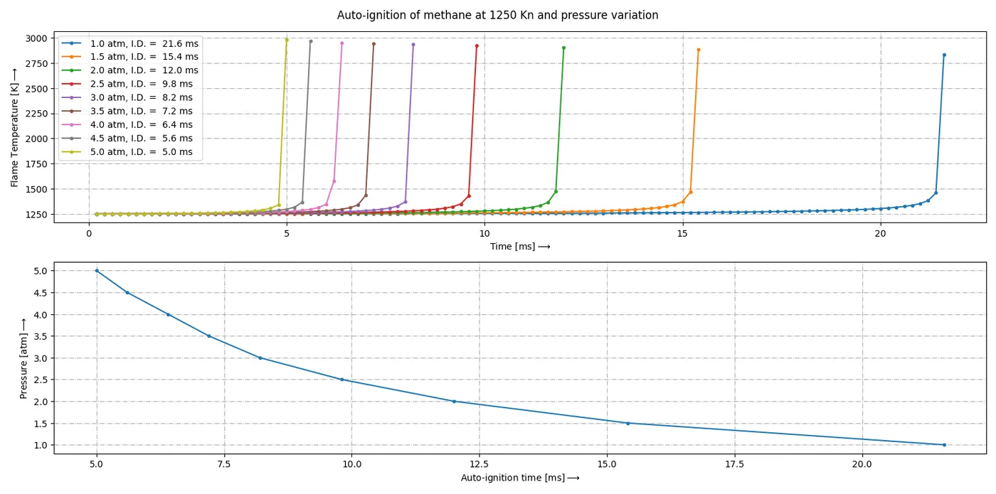
1. The first plot shows the evolution of temperature only till auto-ignition is deemed to occur i.e. until the initial temperature increases by 400K.

2. In the first plot, despite a small time step, ignition causes the temperature to spike so rapidly that the temperature rise curve is not captured adequately. For this, a very small time step will be needed which puts a load on computational resources.

3. Auto-ignition time reduces with an increase in pressure.

4. An increase in pressure increases the collision frequency leading to an increase in reaction rate.

Case 1- B:

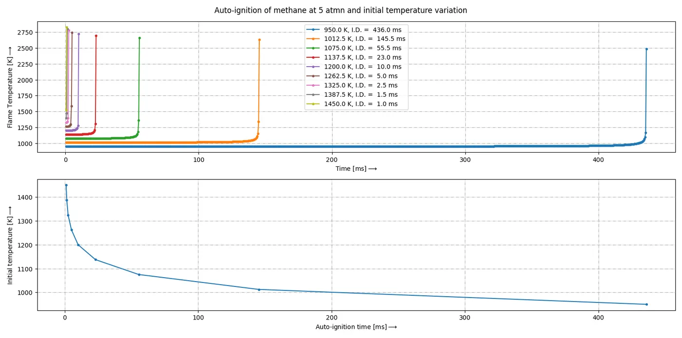
1. Auto-ignition time reduces with increasing initial temperature.

2. This is because as per the Arrhenius equation, the reaction rate varies exponentially with temperature.

3. The trend line shows that auto-ignition time reduces asymptotically with temperature.

Case 2-A and B:

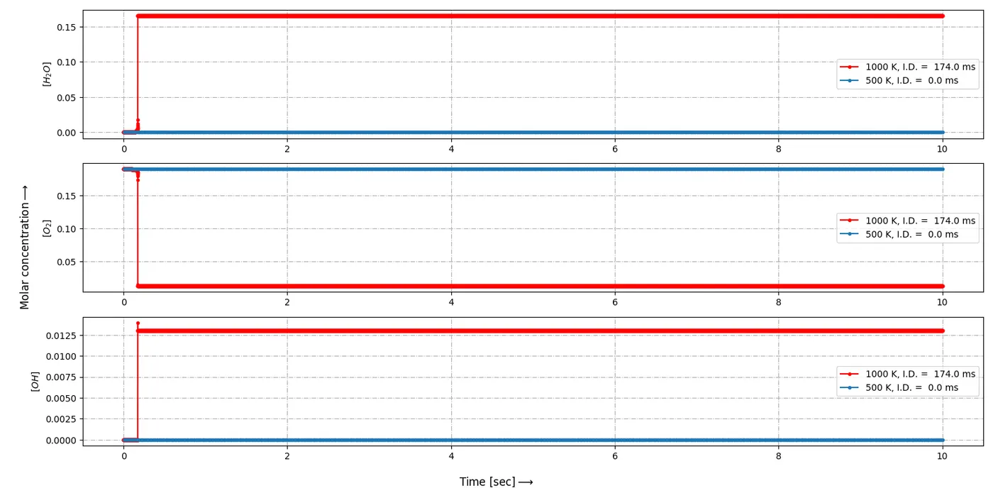
1. At 1000K & 5 atm, OH">OH�� & H2O">H2O�2� concentration rapidly increases while the molar concentration of O2">O2�2 reduces.

2. This indicates the spontaneous combustion of methane.

3. However, at 500K & 5 atm molar concentrations do not change. This is because the pressure & temperature are too low to auto-ignite methane.