Week 7 - Auto ignition using Cantera
AIM:
To study the auto-ignition using cantera.
OBJECTIVE:
To simulate the Auto Ignition Time for Methane under the following conditions, (simulation time = 10 secs)
- Plot the variation of Auto Ignition time of Methane with a constant temperature of 1250K and pressure varying from 1 to 5 atm.
- Plot the variation of Auto Ignition time of Methane with a constant pressure of 5 atm and temperature varying from 950K to 1450K.
- To observe and print the rate of change of molar concentrations of the given elements "H2O, O2, OH" with respect to the time, (simulation time = 10 secs)
Explain the behaviour of the graph for 2 cases,
- When Temperature is 1000K and pressure 5 bar
- When Temperature is 500K and pressure 5 bar
THEORY:
AUTO IGNITION TEMPERATURE:
Auto ignition temperature is the the lowest temperature at which ignition takes place.
Time_(ignition delay) = Time_(initial temperature) + 400k
IGNITION DELAY:
Ignition delay is the time required for ignition to take place. Ignition delay depends on temperature, pressure and mixture composition.
REACTOR:
A Cantera Reactor() represents the simplest form of a chemically reacting system. It corresponds to an extensive thermodynamic control volume V, in which all state variables are homogeneously distributed. The system is generally unsteady — that is, all states are functions of time. In particular, transient state changes due to chemical reactions are possible. However, thermodynamic (but not chemical) equilibrium is assumed to be present throughout the reactor at all instants of time.
Governing Equations for Single Reactors
The state variables for Cantera’s general reactor model are
- m, the mass of the reactor’s contents (in kg)
- V, the reactor volume (in m3)
- A state variable describing the energy of the system, depending on the configuration
- General Reactor(): U, the total internal energy of the reactors contents (in J)
- ConstPressureReactor(): H, the total enthalpy of the reactors contents (in J)
- IdealGasReactor()and IdealGasConstPressureReactor(): T, the temperature (in K)
- Y_k, the mass fractions for each species (dimensionless).
CODING APPROACH:
- A instance gas object is created from solution class and temperature, pressure and moles are set using gas.TPX.
- A reactor object ‘r’ is created using ‘IdealGasReactor’ and gas object is passed to it.
- A reactor network using ‘ReactorNet’ is created by passing the reactor to it.
- A state array is created using SolutionArray for gas.
- ‘Adavance’ command is used to advance the reaction with time.
PART 1:
CASE 1:
PYTHON CODE:
import numpy as np
import cantera as ct
import matplotlib.pyplot as plt

gas = ct.Solution('gri30.xml')
T = 1250
p_min = 1*ct.one_atm
p_max = 5*ct.one_atm
pressure = np.linspace(p_min,p_max,9)
ignition_delay = []
for P in pressure:
	gas.TPX = T,P,{'CH4':1,'O2':2,'N2':7.52}
	r = ct.IdealGasReactor(gas)
	sim = ct.ReactorNet([r])
	time = 0
	states = ct.SolutionArray(gas,extra=['time_in_ms','t'])
	T_old = T
	n = 1
	for n in range(10000):
		time += 1e-3
		sim.advance(time)
		states.append(r.thermo.state,time_in_ms = time*1e3,t = time)
		T_new = states.T
		T_new = T_new[n-1]
		if (T_new>=400+T_old):
			ignition_delay.append(time)
		T_old = states.T
		T_old = T_old[n-1]
	plt.figure(1)
	plt.plot(states.time_in_ms,states.T)
	plt.xlabel('time(ms)')
	plt.ylabel('temperature')
plt.figure(2)
plt.plot(pressure/101325,ignition_delay,'-o')
plt.xlabel('pressure (atm)')
plt.ylabel('ignition delay(ms)')
plt.show()
RESULTS:
TIME VS TEMPERATURE:
PRESSURE VS IGNITION DELAY:
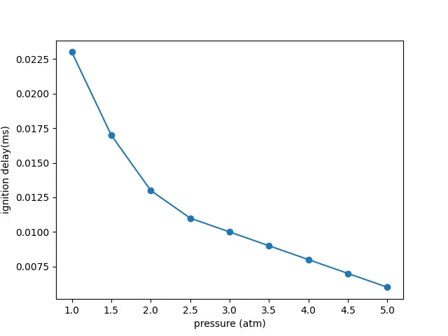
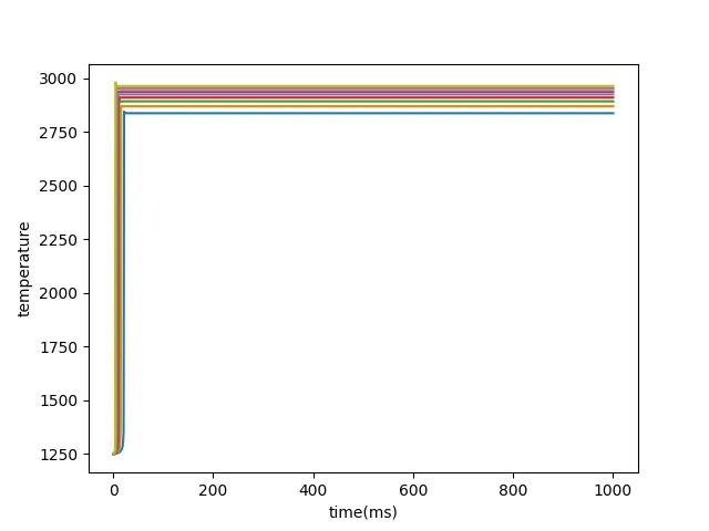
From the above graph we can observe that as initial pressure increases the ignition delay decreases.
CASE 2:
PYTHON CODE:
import numpy as np
import cantera as ct
import matplotlib.pyplot as plt

gas = ct.Solution('gri30.xml')
T_min = 950
T_max = 1450
Temp = np.linspace(T_min,T_max,9)
P = 5*ct.one_atm
ignition_delay = []
for T in Temp:
	gas.TPX = T,P,{'CH4':1,'O2':2,'N2':7.52}
	r = ct.IdealGasReactor(gas)
	sim = ct.ReactorNet([r])
	time = 0
	states = ct.SolutionArray(gas,extra=['time_in_ms','t'])
	T_old = T
	n = 1
	for n in range(10000):
		time += 1e-3
		sim.advance(time)
		states.append(r.thermo.state,time_in_ms = time*1e3,t = time)
		T_new = states.T
		T_new = T_new[n-1]
		if (T_new>=400+T_old):
			ignition_delay.append(time)
		T_old = states.T
		T_old = T_old[n-1]
	plt.figure(1)
	plt.plot(states.time_in_ms,states.T)
	plt.xlabel('time(ms)')
	plt.ylabel('temperature(k)')
	plt.legend(['temp ='+str(T)+'[k]'for T in Temp])
plt.figure(2)
plt.plot(Temp,ignition_delay,'-o')
plt.xlabel('temperature(k)')
plt.ylabel('ignition delay(ms)')
plt.show()
RESULTS:
TIME VS TEMPERATURE:
TEMPERATURE VS IGNITION DELAY:
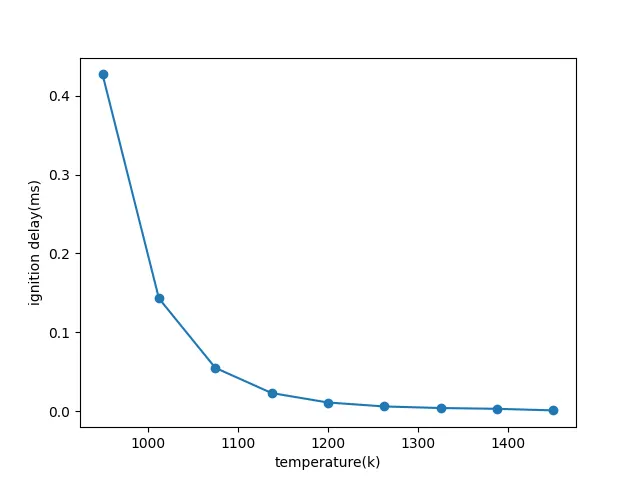
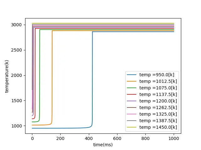
From the above plot we can observe that as initial temperature increases the ignition delay decreases.
So from part 1 we can conclude that the ignition delay is sensitive to both pressure and temperature. as the initial temperature or pressure increases the ignition delay or auto ignition gets reduced.
PART 2:
PYTHON CODE:
import numpy as np
import cantera as ct
import matplotlib.pyplot as plt

gas = ct.Solution('gri30.xml')
T = 1000
P = 5*ct.one_atm
gas.TPX = T,P,{'CH4':1,'O2':2,'N2':7.52}
r = ct.IdealGasReactor(gas)
sim = ct.ReactorNet([r])
time = 0
states = ct.SolutionArray(gas,extra=['time_in_ms','t'])
for n in range(10000):
	time += 1e-3
	sim.advance(time)
	states.append(r.thermo.state,time_in_ms = time*1e3,t = time)
plt.figure(1)
plt.plot(states.time_in_ms,states.X[:,gas.species_index('H2O')])
plt.xlabel('time(ms)')
plt.ylabel('H2O Species')
plt.figure(2)
plt.plot(states.time_in_ms,states.X[:,gas.species_index('O2')])
plt.xlabel('time(ms)')
plt.ylabel('O2 Species')
plt.figure(3)
plt.plot(states.time_in_ms,states.X[:,gas.species_index('OH')])
plt.xlabel('time(ms)')
plt.ylabel('OH Species')
plt.show()
RESULTS:
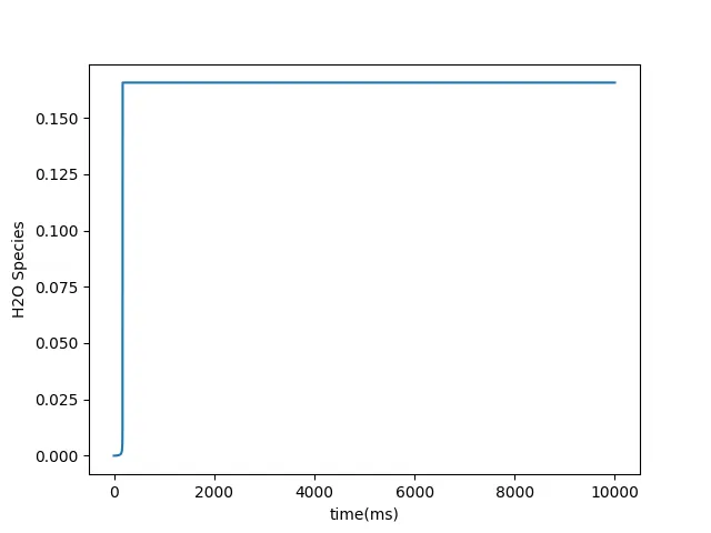
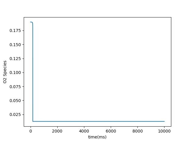
WHEN TEMPERATURE IS 1000K AND PRESSURE 5 BAR:
H2O:
O2:
OH:
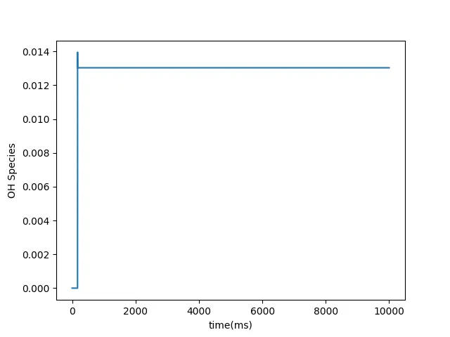
The above plots shows the change in molar concentration of H2O, O2 and OH with a initial temperature and pressure of 1000k and 5 bar.
so from the above plots we can say that after reaction starts there is increases in concentration of H2O and OH and decrease in concentration of O2 which suggest that H2O and OH is formed and O2 is consumed during the combustion process.
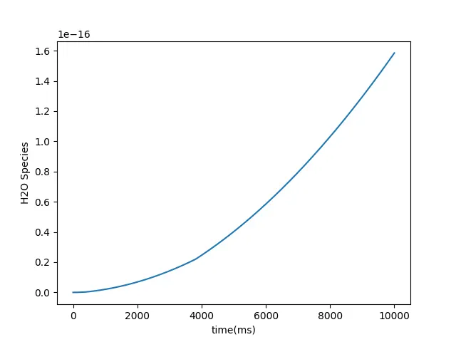
WHEN TEMPERATURE IS 500K AND PRESSURE 5 BAR:
H2O:
O2:
OH:
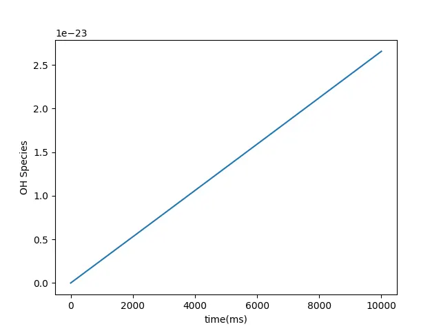
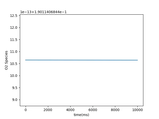
The above plots shows the change in molar concentration of H2O, O2 and OH with a initial temperature and pressure of 500k and 5 bar.
From the O2 plot we can see that for the above case the ignition doesnot takes place because the auto ignition temperature of methane is 900k.
But from the above plots of H2O and OH we can see that the molar concentration of H2O and OH increases due to some intermediate reactions taking place.
REFERENCES: