Week 7 - Auto ignition using Cantera

In this challenge, use the same reactor network code as shown in the video to simulate the Auto Ignition Time for Methane under the following conditions, (simulation time = 10 secs)

• Plot the variation of Auto Ignition time of Methane with a constant temperature of 1250K and pressure varying from 1 to 5 atm.
• Plot the variation of Auto Ignition time of Methane with a constant pressure of 5 atm and temperature varying from 950K to 1450K.

Further, observe and print the rate of change of molar concentrations of the given elements "H2O, O2, OH" with respect to the time, (simulation time = 10 secs)

Explain the behaviour of the graph for 2 cases,

• When Temperature is 1000K and pressure 5 bar
• When Temperature is 500K and pressure 5 bar

Auto Ignition Temperature

The autoignition temperature or kindling point of a substance is the lowest temperature in which it spontaneously ignites in a normal atmosphere without an external source of ignition, such as a flame or spark. This temperature is required to supply the activation energy needed for combustion. The temperature at which a chemical ignites decreases as the pressure or oxygen concentration increases. It is usually applied to a combustible fuel mixture.

Ignition delay is the time gap between fuel injection to the combustion chamber and the very beginning of ignition. The ignition delay can be divided into two, a physical delay and a chemical delay. The physical delay is the time required in atomisation, mixing vaporisation and the chemical delay accounts for the precombustion reaction.

The time for ignition delay can be calculated using the rule that ignition time is the time when the temperature of the reactor is 400K greater than the initial temperature.

Reactor network

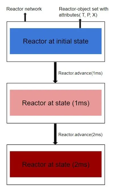
A Cantera reactor is the simplest form of chemical reacting system to generate. It relates to an extensive thermodynamic control volume, in which all state variables are homogeneously distributed. Here all states are a function of time i.e. transient system. The reactor defines the governing equations to be solved. In addition to single reactors, Cantera also owns a facility to interconnect reactors into a Reactor Network. Each reactor in a network may be connected so that the contents of one reactor flow into another. Even for a single reactor, a reactor network is required.

Cantera provides an ODE solver for solving the stiff equations of reacting systems. Starting off the current state of the system it can be advanced (integrate) in a time using a function like ‘advance’. The use of the advance method in a loop has the advantage that it produces results corresponding to a predefined time series. These are associated with predefined memory consumption and well comparable between simulation runs with different parameters.

The Coding Methodology

Case 1:

For analysing the effect of pressure variation on auto-ignition temperature of the methane-air mixture, the temperature is kept at 1250K and pressure is varied between 1 and 5 atm. The temperature-time graph is plotted for different values of pressure and also the ignition delay for different pressures is also calculated.

The Python code using Cantera

import cantera as ct
import matplotlib.pyplot as plt
import numpy as np


T = 1250 #K
ignition_delay =[]

p_min = 1*ct.one_atm
p_max = 5*ct.one_atm
n = 5 

P = np.linspace(p_min,p_max,n)

for j in range(0,len(P)):
	
	gas = ct.Solution('gri30.xml')
	gas.TPX = T, P[j],{'CH4':1,'O2':2,'N2':7.52}
	
	r =ct.IdealGasReactor(gas)
	
	sim = ct.ReactorNet([r])
	
	time = 0.00
	
	states = ct.SolutionArray(gas,extra=['time_in_ms','t'])
	
	Told = T
	
	for k in range(10000):
		time = time +1e-3
		sim.advance(time)
		states.append(r.thermo.state,time_in_ms=time*1e-3,t=time)
		
		Tnew = states.T
		Tnew = Tnew[k-1]
		
		if ((Tnew-Told )> 400):
			ignition_delay.append(time)
			
		Told = states.T
		Told = Told[k-1]
	
	
plt.plot(states.t,states.T)
plt.xlabel('Time (s)')
plt.ylabel('Temperature')
plt.legend(['Pressure -' + str(p)+ '(atm)' for p  in P])
plt.title(r'Temperature v/s Time graph at $T_{initial} = 1250 K$')
plt.grid()
plt.savefig('Time-Temp.png')
plt.show()	
	
	
plt.plot((P/ct.one_atm),ignition_delay,'o-')	
plt.xlabel('Pressure (atm)')
plt.ylabel('Ignition delay (s)')
plt.title(r'Ignition Delay v/s Pressure graph at $T_{initial} = 1250 K$')
plt.grid()
plt.savefig('igntiondelay_pressure.png')
plt.show()

Coding Procedure

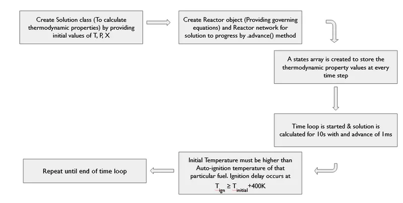
The required libraries are imported. The initial temperature is set to be 1250 K, the pressure value needs to be varied between 1 atm to 5 atm.

An array of pressure is created using the linspace() function. The first for loop is used to vary the pressure in the pressure array.

The IdealGasReactor() method is used to create a reactor that is saved in the variable r.

A reactor network is created using the ReactorNet() command. An array to store the calculated values is created using the SolutionArray() method.

The next for loop is used to change the time for 10 s. The advance() method is used to take the reactor to the next time step.

The ignition delay is calculated by taking the time when the temperature is large by 400K than the initial temperature. The ignition delay values are stored in an array ignition_delay[].

The graphs are plotted using the matplotlib library. In the next part of the challenge instead of pressure, the temperature is stored in an array. In the second part of the challenge the mole fraction of different species are calculated using the command states.X[:,gas.species_index('species')]).

Results

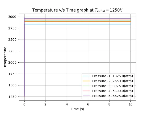
In the above graph, we can observe that as pressure increases we can see that ignition delay decreases.

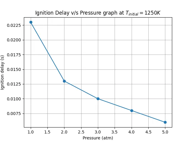
From the above graph, it can be seen that as the pressure increases the ignition delay also decreases. For a very high value of pressure, the ignition delay can be further reduced.

Case 2:

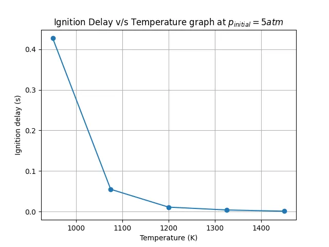
For analysing the effect of temperature variation on auto-ignition temperature of the methane-air mixture, the pressure is kept at 5 atm and temperature is varied between 950 to 1450K. The temperature-time graph is plotted for different values of initial temperature and also the ignition delay for different temperatures is also calculated.

The Python code using Cantera

import cantera as ct
import matplotlib.pyplot as plt
import numpy as np


P = 5*ct.one_atm
ignition_delay =[]

T_min = 950 #K
T_max = 1450 #K
n = 5 

T = np.linspace(T_min,T_max,n)

for j in range(0,len(T)):
	
	gas = ct.Solution('gri30.xml')
	gas.TPX = T[j], P,{'CH4':1,'O2':2,'N2':7.52}
	
	r =ct.IdealGasReactor(gas)
	
	sim = ct.ReactorNet([r])
	
	time = 0.00
	
	states = ct.SolutionArray(gas,extra=['time_in_ms','t'])
	
	Told = T[j]
	
	for k in range(10000):
		time = time +1e-3
		sim.advance(time)
		states.append(r.thermo.state,time_in_ms=time*1e-3,t=time)
		
		Tnew = states.T
		Tnew = Tnew[k-1]
		
		if ((Tnew-Told )>400):
			ignition_delay.append(time)
			
		Told = states.T
		Told = Told[k-1]
	
	
	plt.plot(states.t,states.T)
plt.xlabel('Time (s)')
plt.ylabel('Temperature')
plt.legend(['Temperature -' + str(h)+ 'K' for h  in T])
plt.title(r'Temperature v/s Time graph at $p_{initial} =  5 atm$')
plt.grid()
plt.savefig('Time-Tempatdifftemp.png')	
plt.show()	
	
plt.plot(T,ignition_delay,'o-')	
plt.xlabel('Temperature (K)')
plt.ylabel('Ignition delay (s)')
plt.title(r'Ignition Delay v/s Temperature graph at $p_{initial} = 5 atm$')
plt.grid()
plt.savefig('igntiondelay_press.png')
plt.show()

Results

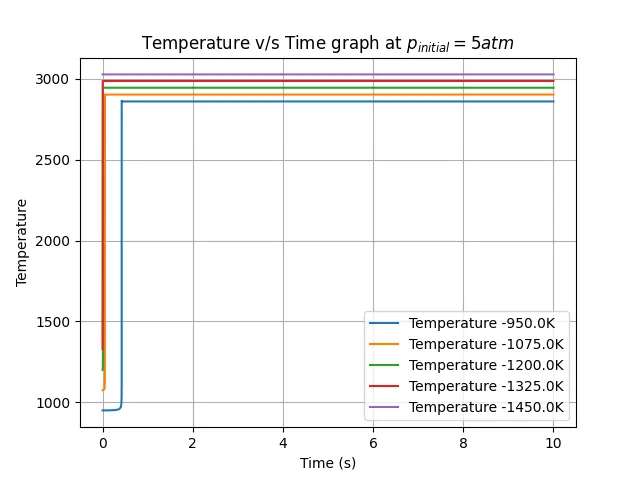
In the above graph, as temperature increases, we can see that ignition delay decreases.

Case 3 :

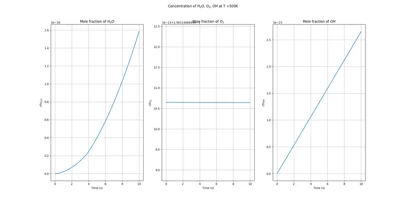
Molar concentrations of the given elements H2O , O2 and OH with respect to the time is calculated for 1000K and 500K and the graphs are plotted.

The Python code using Cantera

import cantera as ct
import matplotlib.pyplot as plt
import numpy as np


P = 5*ct.one_atm
ignition_delay =[]



T = 1000 #K

	
gas = ct.Solution('gri30.xml')
gas.TPX = T, P,{'CH4':1,'O2':2,'N2':7.52}
	
r =ct.IdealGasReactor(gas)
	
sim = ct.ReactorNet([r])
	
time = 0.00
	
states = ct.SolutionArray(gas,extra=['time_in_ms','t'])
	
Told = T
	
for k in range(10000):
	
	time = time +1e-3
	sim.advance(time)
	states.append(r.thermo.state,time_in_ms=time*1e-3,t=time)
		
	Tnew = states.T
	Tnew = Tnew[k-1]
		
	if ((Tnew-Told )>400):
		
		ignition_delay.append(time)
			
	Told = states.T
	Told = Told[k-1]
	
	
	

plt.figure(figsize=(20,10))
plt.subplot(1,3,1)
plt.plot(states.t,states.X[:,gas.species_index('H2O')])
plt.xlabel('Time (s)')
plt.ylabel(r'$chi_{H_2O}$')
plt.title(r'Mole fraction of $H_2O$')
plt.grid()

plt.subplot(1,3,2)
plt.plot(states.t,states.X[:,gas.species_index('O2')])
plt.xlabel('Time (s)')
plt.ylabel(r'$chi_{O_2}$')
plt.title(r'Mole fraction of $O_2$')
plt.grid()

plt.subplot(1,3,3)
plt.plot(states.t,states.X[:,gas.species_index('OH')])
plt.xlabel('Time (s)')
plt.ylabel(r'$chi_{OH}$')
plt.title(r'Mole fraction of $OH$')
plt.suptitle(r'Concentration of $H_2O$, $O_2$, $OH$ at T ='+ str(T) + 'K')
plt.grid()
plt.savefig('moleftraction'+ str(T)+ '.png')
plt.show()

Results

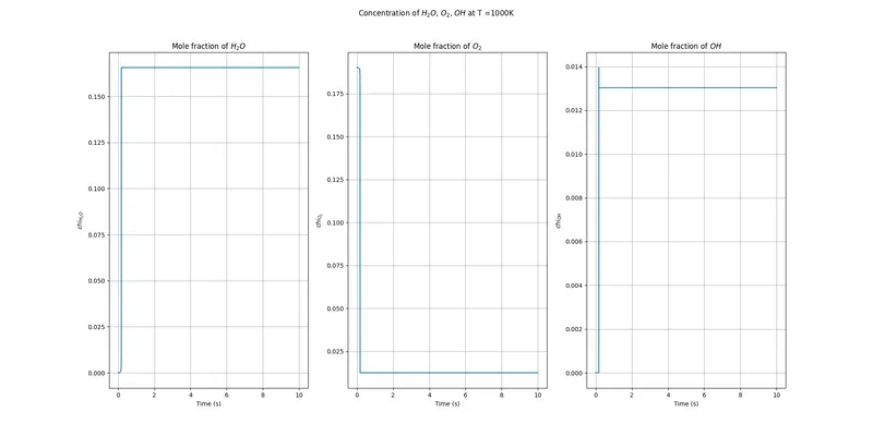
As observed in the above graphs, for the initial temperature of 1000K, the sudden change (spike/drop) in concentration represents the stage of auto-ignition with some ignition delay.

The H2O mole fraction is increased and then stabled throughout the simulation time. This happens due to H2O is the product in methane fuel combustion.

The OH mole fraction is also similar to the H2O, it increases and maintains stability. It is also a product of methane combustion.

The O2 mole fraction is decreased suddenly and maintains stability. The O2 is on the reactant side for the methane combustion and it gets consumed due to further reactions.

For the initial temperature of 500 K, there is no variation in the mole fraction of the oxygen element, where OH and H2O elements vary slightly. This happens due to the bond structures of the molecule. Those are single bond molecules and apparently required less temperature to react or break the bond. Whereas O2 has a double bond and requires more temperature to break the bonds.

Conclusions

As initial pressure increases the ignition delay decreases.

With the increase in initial pressure ignition temperature also increases slightly.

Increment in initial temperature results lowering in ignition delay.

For high initial temperature, ignition temperature is also high and vice versa.

Using 500k as the initial temperature is not ideal as ignition temperature for methane is more than 810K.