Supervised Learning - Classification Week 8 Challenge
Objective: In this project, we will be carrying out the K-nearest neighbours algorithm in the 'Surface defects in steel plates' dataset.
Overview:
Explanation of the K-nearest neighbours algorithm.
Pros and cons of K-Nearest Neighbors.
Performing the KNN algorithm to the dataset.
Summarizing and concluding the observations.
K-Nearest Neighbors Algorithm:
K-nearest neighbours (KNN) algorithm is a type of supervised ML algorithm that can be used for both classifications as well as regression predictive problems. However, it is mainly used for classification predictive problems in the industry. The following two properties would define KNN well −
- Lazy learning algorithm − KNN is a lazy learning algorithm because it does not have a specialized training phase and uses all the data for training while classification.
- Non-parametric learning algorithm − KNN is also a non-parametric learning algorithm because it doesn’t assume anything about the underlying data.
K-nearest neighbours (KNN) algorithm uses ‘feature similarity’ to predict the values of new datapoints which further means that the new data point will be assigned a value based on how closely it matches the points in the training set. We can understand its working with the help of the following steps −
Step 1 − For implementing any algorithm, we need a dataset. So during the first step of KNN, we must load the training as well as test data.
Step 2 − Next, we need to choose the value of K i.e. the nearest data points. K can be any integer.
Step 3 − For each point in the test data do the following −
3.1 − Calculate the distance between test data and each row of training data with the help of any of the methods namely: Euclidean, Manhattan or Hamming distance. The most commonly used method to calculate distance is Euclidean.
3.2 − Now, based on the distance value, sort them in ascending order.
3.3 − Next, it will choose the top K rows from the sorted array.
3.4 − Now, it will assign a class to the test point based on the most frequent class of these rows.
The following is an example to understand the concept of K and working of the KNN algorithm −
Suppose we have a dataset that can be plotted as follows −
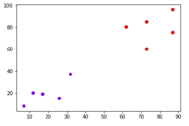
Now, we need to classify new data point with black dot (at point 60,60) into blue or red class. We are assuming K = 3 i.e. it would find three nearest data points. It is shown in the next diagram −
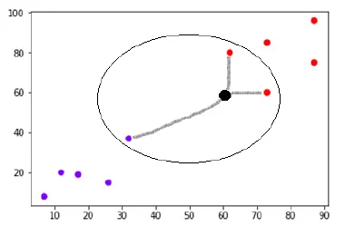
We can see in the above diagram the three nearest neighbours of the data point with a black dot. Among those three, two of them lies in the Red class hence the black dot will also be assigned in the red class.
Advantages and disadvantages of KNN Algorithm
K- Nearest Neighbors or also known as K-NN belong to the family of supervised machine learning algorithms which means we use labelled (Target Variable) dataset to predict the class of new data points. The K-NN algorithm is a robust classifier that is often used as a benchmark for more complex classifiers such as Artificial Neural Network (ANN) or Support vector machine (SVM).
Advantages:
- K-NN is pretty intuitive and simple: K-NN algorithm is very simple to understand and equally easy to implement. To classify the new data point K-NN algorithm reads through the whole dataset to find out K nearest neighbours.
- K-NN has no assumptions: K-NN is a non-parametric algorithm which means there are assumptions to be met to implement K-NN. Parametric models like linear regression have lots of assumptions to be met by data before it can be implemented which is not the case with K-NN.
- No Training Step: K-NN does not explicitly build any model, it simply tags the new data entry based learning from historical data. The new data entry would be tagged with the majority class in the nearest neighbour.
- It constantly evolves: Given its instance-based learning; k-NN is a memory-based approach. The classifier immediately adapts as we collect new training data. It allows the algorithm to respond quickly to changes in the input during real-time use.
- Very easy to implement for the multi-class problem: Most of the classifier algorithms are easy to implement for binary problems and needs the effort to implement for multi-class whereas K-NN adjusts to multi-class without any extra efforts.
- Can be used both for Classification and Regression: One of the biggest advantages of K-NN is that K-NN can be used both for classification and regression problems.
- One Hyper Parameter: K-NN might take some time while selecting the first hyperparameter but after that rest of the parameters are aligned to it.
- Variety of distance criteria to be chosen from: K-NN algorithm gives users the flexibility to choose distance while building a K-NN model. Euclidean Distance, Hamming Distance, Manhattan Distance, Minkowski Distance
Disadvantages:
- K-NN slow algorithm: K-NN might be very easy to implement but as the dataset grows efficiency or speed of the algorithm declines very fast.
- Curse of Dimensionality: KNN works well with a small number of input variables but as the numbers of variables grow K-NN algorithm struggles to predict the output of new data points.
- K-NN needs homogeneous features: If you decide to build k-NN using a common distance, like Euclidean or Manhattan distances, it is completely necessary that features have the same scale, since absolute differences in features weigh the same, i.e., a given distance in feature 1 must mean the same for feature 2.
- An optimal number of neighbours: One of the biggest issues with K-NN is to choose the optimal number of neighbours to be considered while classifying the new data entry.
- Imbalanced data causes problems: k-NN doesn’t perform well on imbalanced data. If we consider two classes, A and B, and the majority of the training data is labelled as A, then the model will ultimately give a lot of preference to A. This might result in getting the less common class B wrongly classified.
- Outlier sensitivity: K-NN algorithm is very sensitive to outliers as it simply chose the neighbours based on distance criteria.
- Missing Value treatment: K-NN inherently has no capability of dealing with the missing value problems.
Performing KNN Classifier on the "Surface defects in Steel plates" dataset:
In this process, we first need to import the data and then start to apply the algorithm.
The classification process will be performed in the following manner:
- Data Preparation and Cleaning.
- Data Visualisation.
- Applying the K-NN algorithm to the dataset.
1. Data preparation and cleaning:
In the first process, we first need to import all the necessary libraries and the dataset on which we are going to perform the algorithm.
import numpy as np
import pandas as pd
import seaborn as sn
import matplotlib.pyplot as plt
df = pd.read_csv('Faults.csv')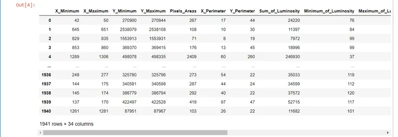
df.describe()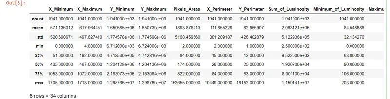
df.info()<class 'pandas.core.frame.DataFrame'>
RangeIndex: 1941 entries, 0 to 1940
Data columns (total 34 columns):
# Column Non-Null Count Dtype
--- ------ -------------- -----
0 X_Minimum 1941 non-null int64
1 X_Maximum 1941 non-null int64
2 Y_Minimum 1941 non-null int64
3 Y_Maximum 1941 non-null int64
4 Pixels_Areas 1941 non-null int64
5 X_Perimeter 1941 non-null int64
6 Y_Perimeter 1941 non-null int64
7 Sum_of_Luminosity 1941 non-null int64
8 Minimum_of_Luminosity 1941 non-null int64
9 Maximum_of_Luminosity 1941 non-null int64
10 Length_of_Conveyer 1941 non-null int64
11 TypeOfSteel_A300 1941 non-null int64
12 TypeOfSteel_A400 1941 non-null int64
13 Steel_Plate_Thickness 1941 non-null int64
14 Edges_Index 1941 non-null float64
15 Empty_Index 1941 non-null float64
16 Square_Index 1941 non-null float64
17 Outside_X_Index 1941 non-null float64
18 Edges_X_Index 1941 non-null float64
19 Edges_Y_Index 1941 non-null float64
20 Outside_Global_Index 1941 non-null float64
21 LogOfAreas 1941 non-null float64
22 Log_X_Index 1941 non-null float64
23 Log_Y_Index 1941 non-null float64
24 Orientation_Index 1941 non-null float64
25 Luminosity_Index 1941 non-null float64
26 SigmoidOfAreas 1941 non-null float64
27 Pastry 1941 non-null int64
28 Z_Scratch 1941 non-null int64
29 K_Scatch 1941 non-null int64
30 Stains 1941 non-null int64
31 Dirtiness 1941 non-null int64
32 Bumps 1941 non-null int64
33 Other_Faults 1941 non-null int64
dtypes: float64(13), int64(21)
memory usage: 515.7 KBNow dividing the data set into 'Faults' and 'Attributes' sets.
Faults = df[['Pastry','Z_Scratch','K_Scatch','Stains','Dirtiness','Bumps','Other_Faults']]
Faults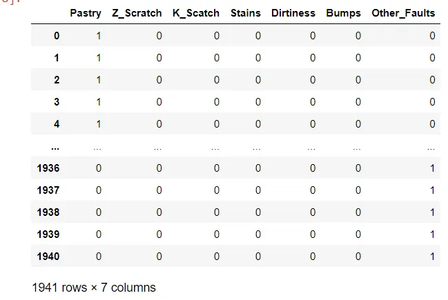
Attributes = df.drop(columns = Faults)
Attributes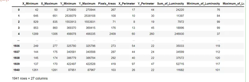
2. Data Visualisation:
In this process, we will check the data how it looks like.
plt.figure(figsize = (15,15))
plt.pie(x=Faults.value_counts().sort_values(),autopct = '%.2f%%',labels = Faults.columns)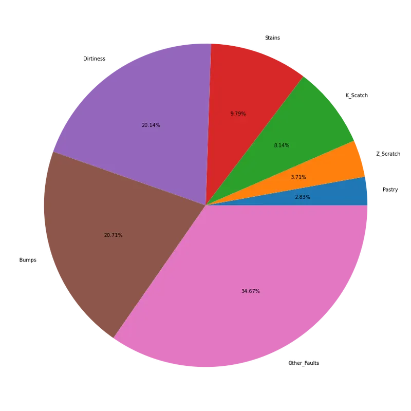
Attributes.hist(figsize = (15,15))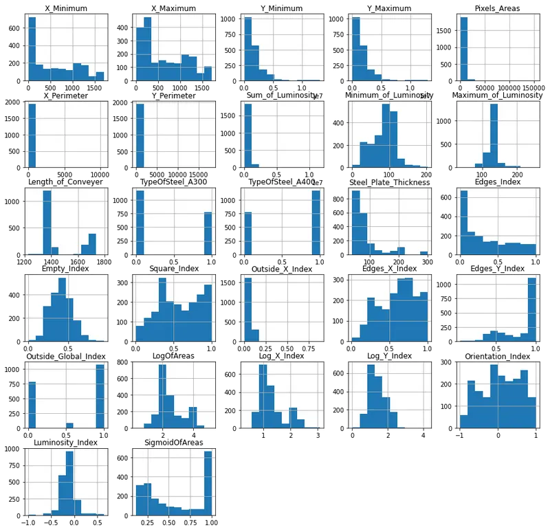
3. Applying the K-NN algorithm:
- In this process, we first import the necessary sklearn libraries for the K-NN algorithm.
- Then we will scale the data as data is too large it is difficult for the processor to run fast.
- After that, we will split the data into test and training subsets.
- Then after we will apply the K-NN algorithm to the dataset.
- We will check the efficiency of the model.
- We will try to predict the test model.
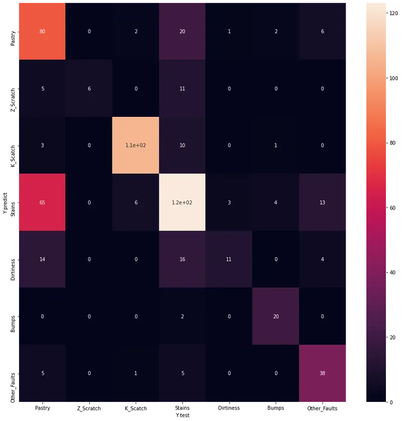
- Lastly, we will create a heatmap of the confusion matrix.
Target = []
for i in range(Faults.shape[0]):
    if df['Pastry'].values[i] == 1:
        Target.append('Pastry')
    elif df['Z_Scratch'].values[i] == 1:
        Target.append('X_Scratch')
    elif df['K_Scatch'].values[i] == 1:
        Target.append('K_Scatch')
    elif df['Stains'].values[i] == 1:
        Target.append('Stains')
    elif df['Dirtiness'].values[i] == 1:
        Target.append('Dirtiness')
    elif df['Bumps'].values[i] == 1:
        Target.append('Bumps')
    else:
        Target.append('Other_Faults')

Target = pd.DataFrame(Target)
df['Target'] = Target
# Scaling the data
from sklearn.preprocessing import StandardScaler
scaler = StandardScaler()
Attributes_scaled = pd.DataFrame(scaler.fit_transform(Attributes),columns = Attributes.columns)
Splitting the data into training and test subset:
from sklearn.model_selection import train_test_split
X_train,X_test,Y_train,Y_test = train_test_split(Attributes_scaled,Target,test_size = 0.3,random_state = 5)
Creating a K-NN classifier model:
from sklearn.neighbors import KNeighborsClassifier
KNN = KNeighborsClassifier(n_neighbors = 40)
Fitting the training data into the model:
KNN.fit(X_train,Y_train)Now we will check for the efficiency of that model.
KNN.score(X_test,Y_test)0.6586620926243568Generating a heatmap of the confusion matrix for this model.
y_predict = KNN.predict(X_test)
from sklearn import metrics

cm = metrics.confusion_matrix(Y_test,y_predict)
cm = pd.DataFrame(cm,columns = Faults.columns)

plt.figure(figsize = (15,15))
sn.heatmap(cm,annot = True,xticklabels = cm,yticklabels = cm)
plt.xlabel('Y test')
plt.ylabel('Y predict')
Discussions and Conclusions:
- The dataset was scaled to avoid long time consumption.
- The value of K was chosen to be 40 after optimization.
- The accuracy of the model was found out to be 65.8%.
- The heatmap of the confusion matrix was generated.