Week 11 - Simulation of Flow through a pipe in OpenFoam
In this challenge, we are going to simulate a laminar flow through the pipe using OpenFOAM. For the ease of simulation time and computational capacity, we are creating a wedge-shaped geometry out of the pipe.
A Matlab code that can generate the computational mesh automatically for any wedge angle and grading schemes is created using file parsing techniques.
Liquids and gasses flowing through circular cross-sectional pipes are one of the most commonly studied phenomena in fluid dynamics. The fluid velocity in a pipe changes from zero at the wall because of the no-slip condition to a maximum at the pipe centre. The characteristics of the flow, whether the flow is laminar, transitional, and turbulent is given by a non-dimensional constant called as the Reynolds number, Re.
For internal flows, we say that the flow is laminar for Re < 2300.
The flow is said to be in transition region for 2300 < Re < 4000.
The flow is turbulent for Re > 4000.
Consider a fluid entering a circular pipe at a uniform velocity.
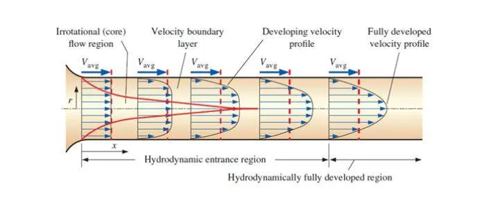
Because of the no-slip condition, the fluid particles in the layer in contact with the wall of the pipe come to a complete stop. This layer also causes the fluid particles in the adjacent layers to slow down gradually as a result of friction. To make up for this velocity reduction, the velocity of the fluid at the mid-section of the pipe has to increase to keep the mass flow rate through the pipe constant. As a result, a velocity gradient develops along the pipe.
The region of the flow in which the effects of the viscous shearing forces caused by fluid viscosity are felt is called the boundary layer. The hypothetical boundary surface divides the flow in a pipe into two regions: the boundary layer region, in which the viscous effects and the velocity changes are significant, and the irrotational (core) flow region, in which the frictional effects are negligible and the velocity remains essentially constant in the radial direction.
The thickness of this boundary layer increases in the flow direction until the boundary layer reaches the pipe centre and thus fills a region of the pipe and the velocity becomes fully developed a little farther downstream.
The region from the pipe inlet to the point at which the velocity profile is fully developed is called the hydrodynamic entrance region, and the length of this region is called the hydrodynamic entry length. Flow in the entrance region is called hydrodynamically developing flow since this is the region where the velocity profile develops. The region beyond the entrance region in which the velocity profile is fully developed and remains unchanged is called the hydrodynamically fully developed region.
Hagen–Poiseuille equation
The Hagen–Poiseuille equation, also known as the Hagen–Poiseuille law, is a physical law that gives the pressure drop in an incompressible and Newtonian fluid in laminar flow flowing through a long cylindrical pipe of constant cross-section.
Assumptions:
- The fluid is incompressible and Newtonian.
- The flow is laminar through a pipe of the constant circular cross-section that is substantially longer than its diameter.
- There is no acceleration of fluid in the pipe.
The relations that are given by the Hagen–Poiseuille equation is given below.
Velocity profileis given by the equation,
`u(r) = 2*V_(avg)*[1-frac(r^2)(R^2)]`
By substitutiong `r = R`, we get `u(R) = V_(max) = 2*V_(avg)`.
The entrance length, `L_h approx 0.06*R_e*D`
The pressure drop, `Delta P = P_1-P_2 = frac (32*mu*L*V_(avg))(D^2)`
Shear stress, `tau = mu* frac(delu)(dely)`
Computational Wedge
The computational wedge is given below. The wedge angle should be less than 5 degrees. We have to make sure that the number of cells along the axisymmetric.
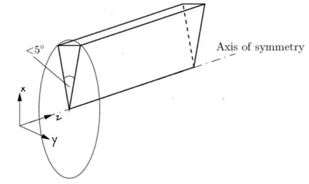
The numbering of the vertices is given by the figure,
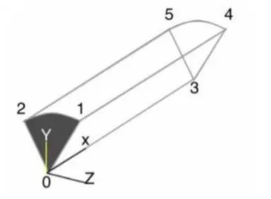
Properties that are associated with the simulation is given by,
Working fluid: Water at `25°` C
Reynold's number: Re = 2000, Laminar flow.
Dynamic viscosity: 8.9e-04 `frac (Ns)(m^2)` at 25° C
Kinematic Viscosity: 8.9268e-07
The diameter of pipe: 0.015 m
The density of water: 997 kg/m3
Length required to fully developed flow: L = `L_e` + 0.3 .
`Re = (VrhoD)/mu`, V = 0.119 m/s
MATLAB code to generate a computational blockMeshDict file automatically for any wedge angle by using file parsing technique.
clear all
close all
clc

% Reynolds number
re=2000;
% Diameter of pipe
d=0.015;
% Radius
r=d/2;
% Calculating enterance length based on diameter & Re
le=0.05*re*d;
% Density of water
rho=997;
% Dynamic viscosity of water
mu=0.00089;
% Wedge angle (<5)
theta=4;
% Kinematic viscosity
nu=mu/rho;
v_avg=(re*mu)/(rho*d);
% Maximum velocity
v_max=2*v_avg;
% Total length
l=le+1;
% Hagen Poiseulle equation
deltap=(32*mu*l*v_avg)/(d)^2;
% Kinematic pressure
kinematic_p=deltap/rho;
% Courant number = 0.45
deltat= (0.45*(l/200))/v_avg+(0.45*(r/20))/v_avg;

% blockMesh file generation
f1=fopen('blockMeshDict','w')

fprintf(f1,'FoamFile\n{\n')
fprintf(f1,'%12s \t 2.0;\n','version')
fprintf(f1,'%12s \t ascii;\n','format');
fprintf(f1,'%12s \t dictionary;\n','class');
fprintf(f1,'%12s \t blockMeshDict;\n)\n\n','object');

fprintf(f1,'convertToMeters 1;\n\n')

fprintf(f1,'vertices\n(\n')
fprintf(f1,'\t (%d %d %d)\n',0,0,0);
fprintf(f1,'\t (%d %d %d)\n',0,r*cosd(theta/2),r*sind(theta/2))
fprintf(f1,'\t (%d %d %d)\n',0,r*cosd(theta/2),-r*sind(theta/2))
fprintf(f1,'\t (%d %d %d)\n',l,0,0)
fprintf(f1,'\t (%d %d %d)\n',l,r*cosd(theta/2),r*sind(theta/2))
fprintf(f1,'\t (%d %d %d)\n',l,r*cosd(theta/2),-r*sind(theta/2))
fprintf(f1,');\n\n')

fprintf(f1,'blocks\n(\n')
fprintf(f1,'\t hex (0 3 5 2 0 3 4 1) (%d %d %d)',200,20,1)
fprintf(f1,' SimpleGrading (1 0.1 1)\n\n);\n\n')

fprintf(f1,'edges\n(\n')
fprintf(f1,'\t arc %d %d (%d %d %d)\n',1,2,0,r,0)
fprintf(f1,'\t arc %d %d (%d %d %d)\n',4,5,l,r,0)
fprintf(f1,');\n\n')

fprintf(f1, 'boundary\n')
fprintf(f1,'(\n')
fprintf(f1,'\t inlet\n')
fprintf(f1,'\t {\n')
fprintf(f1,'\t\t type patch;\n')
fprintf(f1,'\t\t faces\n')
fprintf(f1,'\t\t (\n')
fprintf(f1,'\t\t\t (0 1 2 0)\n\t\t);\n')
fprintf(f1,'\t }\n')

fprintf(f1,'\t outlet\n')
fprintf(f1,'\t {\n')
fprintf(f1,'\t\t type patch;\n')
fprintf(f1,'\t\t faces\n\t\t(\n')
fprintf(f1,'\t\t\t (3 5 4 3)\n\t\t);\n')
fprintf(f1,'\t }\n')

fprintf(f1,'\t top\n')
fprintf(f1,'\t {\n')
fprintf(f1,'\t\t type wall;\n')
fprintf(f1,'\t\t faces\n\t\t(\n')
fprintf(f1,'\t\t\t (1 4 5 2)\n\t\t);\n')
fprintf(f1,'\t }\n')

fprintf(f1,'\t front\n')
fprintf(f1,'\t {\n')
fprintf(f1,'\t\t type wedge;\n')
fprintf(f1,'\t faces\n\t\t(\n')
fprintf(f1,'\t\t\t (0 3 4 1)\n\t\t);\n')
fprintf(f1,'\t }\n')

fprintf(f1,'\t back\n')
fprintf(f1,'\t {\n')
fprintf(f1,'\t\t type wedge;\n')
fprintf(f1,'\t faces\n\t\t(\n')
fprintf(f1,'\t\t\t (0 2 5 3)\n\t\t);\n')
fprintf(f1,'\t }\n')

fprintf(f1,'\t axis\n')
fprintf(f1,'\t {\n')
fprintf(f1,'\t\t type empty;\n')
fprintf(f1,'\t faces\n\t\t(\n')
fprintf(f1,'\t\t\t (0 3 3 0)\n\t\t);\n')
fprintf(f1,'\t }\n')
fprintf(f1,');\n')

fprintf(f1,'mergePatchPairs\n')
fprintf(f1,'(\n);\n')


fclose(f1)
The generated blockMeshDict file:
FoamFile
{
     version 	 2.0;
      format 	 ascii;
       class 	 dictionary;
      object 	 blockMeshDict;
)

convertToMeters 1;

vertices
(
	 (0 0 0)
	 (0 7.495431e-03 2.617462e-04)
	 (0 7.495431e-03 -2.617462e-04)
	 (2.500000e+00 0 0)
	 (2.500000e+00 7.495431e-03 2.617462e-04)
	 (2.500000e+00 7.495431e-03 -2.617462e-04)
);

blocks
(
	 hex (0 3 5 2 0 3 4 1) (200 20 1) SimpleGrading (1 0.1 1)

);

edges
(
	 arc 1 2 (0 7.500000e-03 0)
	 arc 4 5 (2.500000e+00 7.500000e-03 0)
);

boundary
(
	 inlet
	 {
		 type patch;
		 faces
		 (
			 (0 1 2 0)
		);
	 }
	 outlet
	 {
		 type patch;
		 faces
		(
			 (3 5 4 3)
		);
	 }
	 top
	 {
		 type wall;
		 faces
		(
			 (1 4 5 2)
		);
	 }
	 front
	 {
		 type wedge;
	 faces
		(
			 (0 3 4 1)
		);
	 }
	 back
	 {
		 type wedge;
	 faces
		(
			 (0 2 5 3)
		);
	 }
	 axis
	 {
		 type empty;
	 faces
		(
			 (0 3 3 0)
		);
	 }
);
mergePatchPairs
(
);

// ************************************************************************* //
controlDict file:
/*--------------------------------*- C++ -*----------------------------------*\
  =========                 |
  \\      /  F ield         | OpenFOAM: The Open Source CFD Toolbox
   \\    /   O peration     | Website:  https://openfoam.org
    \\  /    A nd           | Version:  8
     \\/     M anipulation  |
\*---------------------------------------------------------------------------*/
FoamFile
{
    version     2.0;
    format      ascii;
    class       dictionary;
    location    "system";
    object      controlDict;
}
// * * * * * * * * * * * * * * * * * * * * * * * * * * * * * * * * * * * * * //

application     icoFoam;

startFrom       startTime;

startTime       0;

stopAt          endTime;

endTime         50;

deltaT          0.02;

writeControl    timeStep;

writeInterval   20;

purgeWrite      0;

writeFormat     ascii;

writePrecision  6;

writeCompression off;

timeFormat      general;

timePrecision   6;

runTimeModifiable true;


// ************************************************************************* //
Initial condition:
Pressure(p)
/*--------------------------------*- C++ -*----------------------------------*\
  =========                 |
  \\      /  F ield         | OpenFOAM: The Open Source CFD Toolbox
   \\    /   O peration     | Website:  https://openfoam.org
    \\  /    A nd           | Version:  8
     \\/     M anipulation  |
\*---------------------------------------------------------------------------*/
FoamFile
{
    version     2.0;
    format      ascii;
    class       volScalarField;
    object      p;
}
// * * * * * * * * * * * * * * * * * * * * * * * * * * * * * * * * * * * * * //

dimensions      [0 2 -2 0 0 0 0];

internalField   uniform 0;

boundaryField
{
    inlet
    {
        type            zeroGradient;
    }

    outlet
    {
        type            fixedValue;
        value           uniform 0;
    }

    axis
    {
        type            empty;
    }

    top
    {
        type            zeroGradient;
    }

    front
    {
        type            wedge;
    }

    back
    {
        type            wedge;
    }
}

// ************************************************************************* //
Velocity (U)
/*--------------------------------*- C++ -*----------------------------------*\
  =========                 |
  \\      /  F ield         | OpenFOAM: The Open Source CFD Toolbox
   \\    /   O peration     | Website:  https://openfoam.org
    \\  /    A nd           | Version:  8
     \\/     M anipulation  |
\*---------------------------------------------------------------------------*/
FoamFile
{
    version     2.0;
    format      ascii;
    class       volVectorField;
    object      U;
}
// * * * * * * * * * * * * * * * * * * * * * * * * * * * * * * * * * * * * * //

dimensions      [0 1 -1 0 0 0 0];

internalField   uniform (0 0 0);

boundaryField
{
    inlet
    {
        type            fixedValue;
        value           uniform (0.1190 0 0);
    }

    outlet
    {
        type            zeroGradient;
    }

    axis
    {
        type            empty;
    }

    top
    {
        type            fixedValue;
        value           uniform (0 0 0);
    }

    front
    {
        type            wedge;
    }

    back
    {
        type            wedge;
    }
}

// ************************************************************************* //
tansportProperties
/*--------------------------------*- C++ -*----------------------------------*\
  =========                 |
  \\      /  F ield         | OpenFOAM: The Open Source CFD Toolbox
   \\    /   O peration     | Website:  https://openfoam.org
    \\  /    A nd           | Version:  8
     \\/     M anipulation  |
\*---------------------------------------------------------------------------*/
FoamFile
{
    version     2.0;
    format      ascii;
    class       dictionary;
    location    "constant";
    object      transportProperties;
}
// * * * * * * * * * * * * * * * * * * * * * * * * * * * * * * * * * * * * * //

nu              [0 2 -1 0 0 0 0] 8.9268e-07;


// ************************************************************************* //
Results:
The generated mesh is given below,
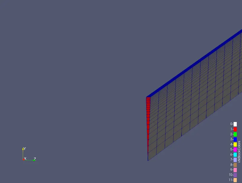
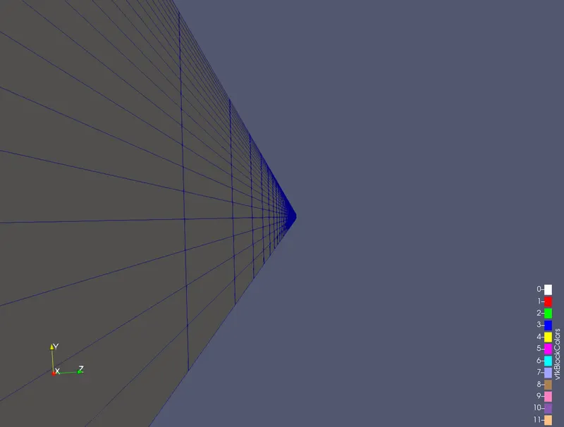
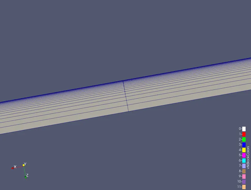
Hydrodynamic Entrance Length: 1.5m, Total length = 1+1.5 = 2.5 m
We have given 200 divisions along the length of the pipe and 20 divisions along the radial distance. With simple grading of 0.1 in the y-direction.
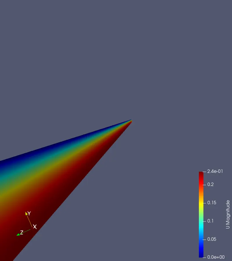
Velocity distribution along the wedge is given by,
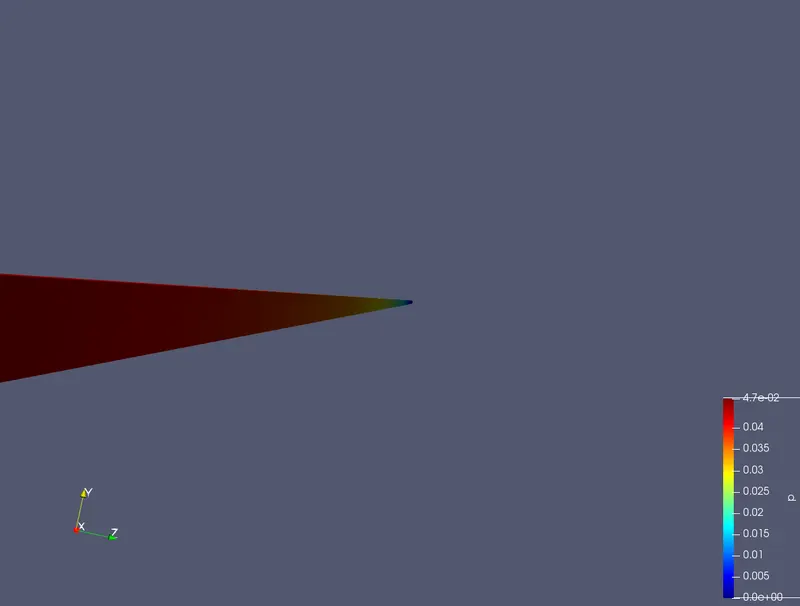
The pressure distribution is given by,
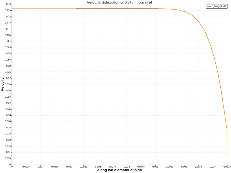
Velocity profile at a distance 0.01 m from the inlet along the radial distance is given by,
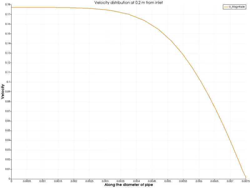
Velocity profile at a distance 0.2 m from the inlet along the radial distance is given by,
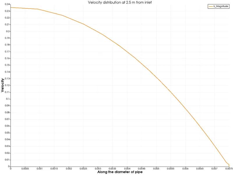
Velocity profile at a distance 2.5 m from the inlet along the radial distance is given by,
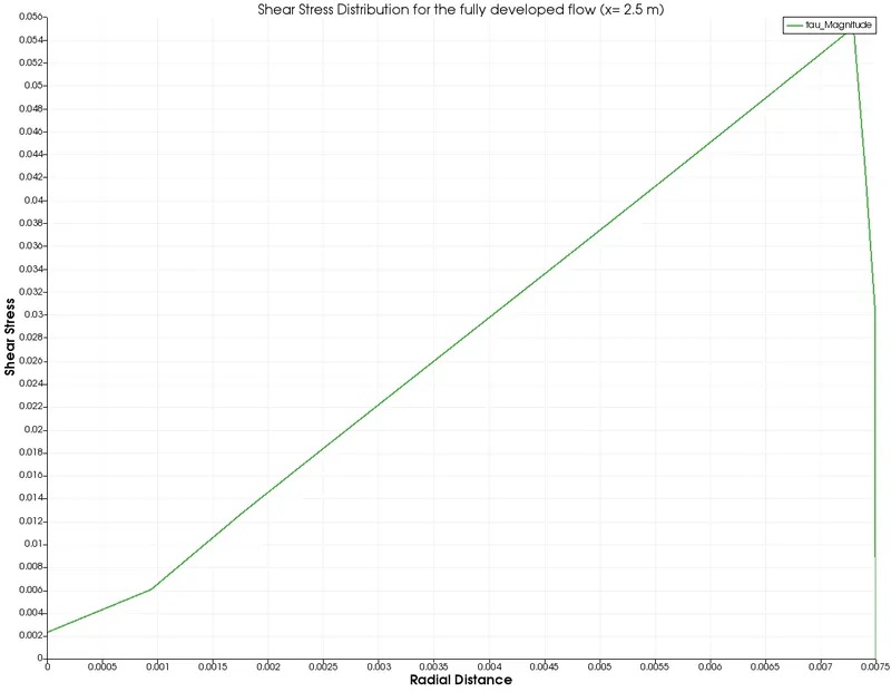
Shear stress distribution at a distance 2.5 m from the inlet along the radial distance is given by,
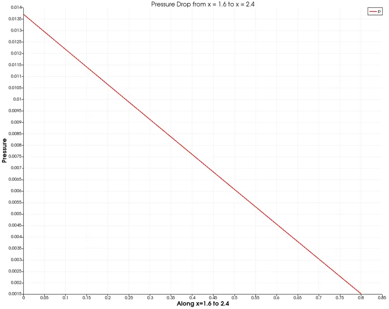
The pressure drop from x = 1.6 m to x = 2.5,
Validation
| Parameter | Theoretical value | Computed value | Percentage Error |
| Maximum Velocity (`V_(max)`) | 0.238047 | 0.230183 | 3.3% |
| Pressure Drop from 1.6 m to 2.4 m. (`Delta p`) | 0.012086 | 0.01215744 | 0.59% |
| Shear Stress (`tau`) | 0.0564964 | 0.055074 | 2.51% |
Discussion and Conclusions
The Hagen–Poiseuille equation was validated with the simulation results.
It can be observed from in the velocity profiles that the flow which is initially at the irrotational region develops to the fully developed region at the outlet. At x=0.01 m and x= 0.2 m, which lies in the hydrodynamic entrance length, the flow develops accordingly. At x =2.5 m from the inlet, the flow is fully developed.
The pressure drop from x = 1.6 m to x = 2.4(Following the hydrodynamic entrance region)numerical results we see that the percentage error is very less for the pressure drop across the region.
As the error is less 5% for the flow parameters, the model can be said to be validated.