Week 7 - Auto ignition using Cantera

AIM:

Part-1: To simulate the Auto Ignition Time for Methane under the following conditions, (simulation time = 10 secs)

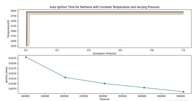
• To plot the variation of Auto Ignition time of Methane with a constant temperature of 1250K and pressure varying from 1 to 5 atm.
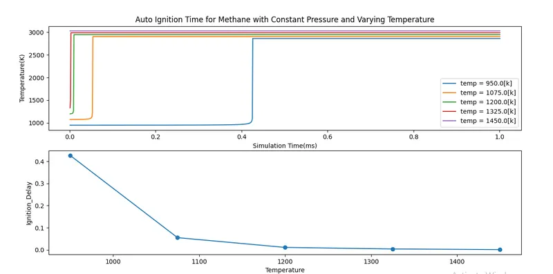
• To plot the variation of Auto Ignition time of Methane with a constant pressure of 5 atm and temperature varying from 950K to 1450K.

Part-2:

To observe and print the rate of change of molar concentrations of "H2O, O2, OH" with respect to the time, (simulation time = 10 secs)

Explain the behavior of the graph for 2 cases,

• When Temperature is 1000K and pressure 5 bar
• When Temperature is 500K and pressure 5 bar

Introduction:

Auto Ignition:

The autoignition temperature or kindling point of a substance is the lowest temperature in which it spontaneously ignites in a normal atmosphere without an external source of ignition, such as a flame or spark.

This temperature is required to supply the activation energy needed for combustion. The temperature at which a chemical ignites decreases as the pressure or oxygen concentration increases. It is usually applied to a combustible fuel mixture.

• The ignition temperature of a substance is the least temperature at which the substance starts combustion.
• Substances which spontaneously ignite in a normal atmosphere at naturally ambient temperatures are termed pyrophoric.

Temperatures vary widely in the literature and should only be used as estimates. Factors that may cause variation include partial pressure of oxygen, altitude, humidity, and amount of time required for ignition. Generally the autoignition temperature for hydrocarbon/air mixtures decreases with increasing molecular mass and increasing chain length. The autoignition temperature is also higher for branched-chain hydrocarbons than for straight-chain hydrocarbons.

Auto Ignition time is the time when the temperature of the reactor is Initial Temperature plus 400K.

Ignition Delay:

The ignition delay in a diesel engine is defined as the time interval between the start of injection and the start of combustion.

This delay period consists of

(a) physical delay, wherein atomisation, vaporization and mixing of air fuel occur
(b) of chemical delay attributed to pre-combustion reactions.

Physical and chemical delays occur simultaneously. To reduce NOx, the method adapted in modern engines is to reduce the ignition delay.

Part-1:

Simulation of Auto Ignition Time for Methane by varying temperature and pressure.

Case-1: Constant Temperature(1250K) & Pressure(1 - 5 atm)

"""
Simulation of Auto Ignition Time for Methane with Constant Temperature and Varying Pressure
"""

import numpy as np
import cantera as ct
import sys
import matplotlib.pyplot as plt

gas = ct.Solution('gri30.xml')
p_start = ct.one_atm
p_end = ct.one_atm*5

pressure = np.linspace(p_start,p_end,5)
ignition_delay = []

for i in range(1,6):

	# Pressure varying from 1atm to 5atm
	P = ct.one_atm*i
	# Temperature
	T = 1250
	gas.TPX = T,P,{'CH4':1,'O2':2,'N2':7.52}
	r = ct.IdealGasReactor(gas)
	sim = ct.ReactorNet([r]) # Reactor Network
	time = 0
	sim_time = 10*100
	
	states = ct.SolutionArray(gas,extra=['time_in_ms','t'])
	T_old = T

	for j in range(sim_time+1):
		time+= 1e-3
		sim.advance(time) # Advancing the solution with respect to time step
		states.append(r.thermo.state, time_in_ms = time*1e-3, t = time)

		T_new = states.T
		T_new = T_new[j-1]

		if (T_new - T_old) >= 400:
			ignition_delay.append(time)

		T_old = states.T
		T_old = T_old[j-1]

	plt.subplot(2,1,1)	
	plt.plot(states.t,states.T)
	plt.xlabel('Simulation Time(ms)')
	plt.ylabel('Temperature(K)')
	plt.title('Auto Ignition Time for Methane with Constant Temperature and Varying Pressure')
	
plt.subplot(2,1,2)
plt.plot(pressure,ignition_delay,'-o')
plt.xlabel('Pressure')
plt.ylabel('Ignition_Delay')
plt.show()

Results:

Case-2: Constant pressure(5 atm) & Temperature(950K - 1450K).

"""
Simulation of Auto Ignition Time for Methane with Constant Pressure and Varying Temperature
"""

import numpy as np
import cantera as ct
import matplotlib.pyplot as plt

gas = ct.Solution('gri30.xml')
T_start = 950
T_end = 1450

temp = np.linspace(T_start,T_end,5)
ignition_delay = []

for i in range(len(temp)):

	# Pressure varying from 1atm to 5atm
	P = ct.one_atm*5
	
	gas.TPX = temp[i],P,{'CH4':1,'O2':2,'N2':7.52}
	r = ct.IdealGasReactor(gas)
	sim = ct.ReactorNet([r]) # Reactor Network
	time = 0
	sim_time = 10*100
	
	states = ct.SolutionArray(gas,extra=['time_in_ms','t'])
	T_old = temp[i]

	for j in range(sim_time+1):
		time+= 1e-3
		sim.advance(time) # Advancing the solution with respect to time step
		states.append(r.thermo.state, time_in_ms = time*1e-3, t = time)

		T_new = states.T
		T_new = T_new[j-1]

		if (T_new - T_old) >= 400:
			ignition_delay.append(time)

		T_old = states.T
		T_old = T_old[j-1]

	plt.subplot(2,1,1)	
	plt.plot(states.t,states.T)
	plt.xlabel('Simulation Time(ms)')
	plt.ylabel('Temperature(K)')
	plt.title('Auto Ignition Time for Methane with Constant Pressure and Varying Temperature')
	plt.legend(['temp = '+str(T) +'[k]' for T in temp])
	
plt.subplot(2,1,2)
plt.plot(temp,ignition_delay,'-o')
plt.xlabel('Temperature')
plt.ylabel('Ignition_Delay')
plt.show()

Results:

Part-2: The rate of change of molar concentrations of "H2O, O2, OH"

"""
Simulation of the rate of change of molar concentrations of "H2O, O2, OH"
"""

import numpy as np
import cantera as ct
import matplotlib.pyplot as plt


temp = [1000,500]

for T in temp:

	gas = ct.Solution('gri30.xml')
	# Pressure varying from 1atm to 5atm
	P = ct.one_atm*5
	
	gas.TPX = T,P,{'CH4':1,'O2':2,'N2':7.52}
	r = ct.IdealGasReactor(gas)
	sim = ct.ReactorNet([r]) # Reactor Network
	time = 0
	sim_time = 10*100
	
	states = ct.SolutionArray(gas,extra=['time_in_ms','t'])
	T_old = T

	for j in range(sim_time+1):
		time+= 1e-3
		sim.advance(time) # Advancing the solution with respect to time step
		states.append(r.thermo.state, time_in_ms = time*1e-3, t = time)


	plt.subplot(3,1,1)	
	plt.plot(states.t,states.X[:,gas.species_index('H2O')])
	plt.xlabel('Simulation Time(ms)')
	plt.ylabel('H2O_Molefraction')
	
	plt.subplot(3,1,2)	
	plt.plot(states.t,states.X[:,gas.species_index('O2')])
	plt.xlabel('Simulation Time(ms)')
	plt.ylabel('O2_Molefraction')
	
	plt.subplot(3,1,3)	
	plt.plot(states.t,states.X[:,gas.species_index('H2O')])
	plt.xlabel('Simulation Time(ms)')
	plt.ylabel('OH_Molefraction')
	plt.show()

Results:

Case-1: Temperature(1000K) & Pressure(5atm)

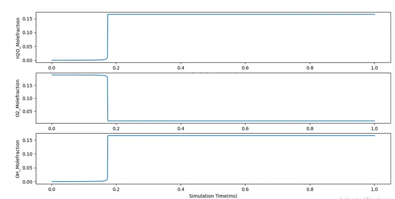
H2O concentration is very low before auto ignition and after auto ignition it increases and remains constant.

O2 after auto ignition decreases as it reacts with fuel.

OH is less and after auto ignition increases.

Case-2: Temperature(500K) & Pressure(5atm)

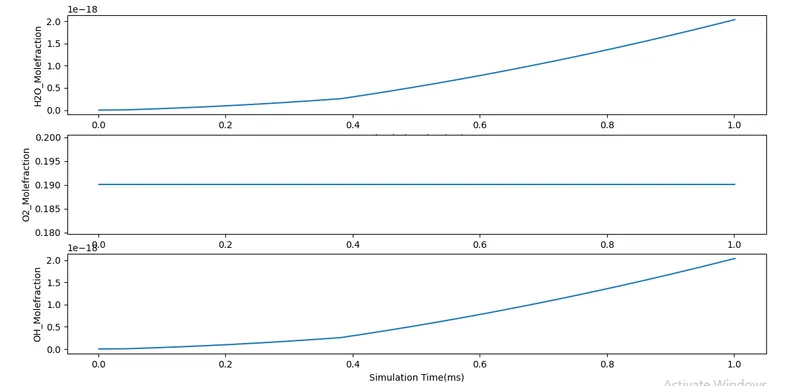
As we know that Methane auto ignites at 873K, hence combustion doesnot take place. So, the O2 remains constant.

The H2O & OH changes because of ambient reactions.

Conclusion:

The initial temperature is important to start the combustion process. And this depends on the fuel we use. Here, due to less temperature(500K & Methane) combustion does not take place.