Week 6 - Multivariate Newton Rhapson Solver

AIM:-

This project aims to solve the system of ODE using the Newton-Raphson method.

Python Program:-

"""
This python program is written to solve a system of coupled non-linear equations
using multivariate Newton-Raphson solver

dy1/dt = -0.04*y1 + 10^4*y2*y3
dy2/dt = 0.04*y1 - 10^4y2*y3 - 3.10^7*y2^2
dy3/dt = 3.10^7*y2^2

"""

import matplotlib.pyplot as plt
import numpy as np
from numpy.linalg import inv

#Time interval definition

t_start = 0
t_end = 600
dt = 0.01
n = int((t_end-t_start)/dt)




def f1(y1_old, y1, y2, y3, dt):

	# First non-linear equation 
	return y1_old + dt*(-0.04*y1 + 1*10**4*y2*y3) - y1


def f2(y2_old, y1, y2, y3, dt):
	#Second non-linear equation

	return y2_old + dt*(0.04*y1 - 10**4*y2*y3 - 3*10**7*y2**2) - y2

def f3(y3_old, y1, y2, y3, dt):

	# Third non-linear equation

	return y3_old + dt*(3*10**7*y2**2) - y3

def Jacobian(y1_old, y2_old, y3_old, y1, y2, y3, dt):
	J = np.ones((3,3))
	h = 1e-5
	# Row 1
	J[0,0] = (f1(y1_old, y1+h, y2, y3, dt) - f1(y1_old, y1, y2, y3, dt))/h
	J[0,1] = (f1(y1_old, y1, y2+h, y3, dt) - f1(y1_old, y1, y2, y3, dt))/h
	J[0,2] = (f1(y1_old, y1+h, y2, y3+h, dt) - f1(y1_old, y1, y2, y3, dt))/h

	# Row 2
	J[1,0] = (f2(y2_old, y1+h, y2, y3, dt) - f2(y2_old, y1, y2, y3, dt))/h;
	J[1,1] = (f2(y2_old, y1, y2+h, y3, dt) - f2(y2_old, y1, y2, y3, dt))/h;
	J[1,2] = (f2(y2_old, y1, y2, y3+h, dt) - f2(y2_old, y1, y2, y3, dt))/h;

	# Row 3
	J[2,0] = (f3(y3_old, y1+h, y2, y3, dt) - f3(y3_old, y1, y2, y3, dt))/h;
	J[2,1] = (f3(y3_old, y1, y2+h, y3, dt) - f3(y3_old, y1, y2, y3, dt))/h;
	J[2,2] = (f3(y3_old, y1, y2, y3+h, dt) - f3(y3_old, y1, y2, y3, dt))/h;

	return J



#Initial guess values definition

y1_old = 1
y2_old = 0
y3_old = 0


#Defining the column vector

Y_old = np.ones((3,1))
Y_old[0] = y1_old
Y_old[1] = y2_old
Y_old[2] = y3_old
#Defining the guess values column vector



F = np.copy(Y_old)

#Defining the initial error
error = 9e9

alpha = 1

tol = 1e-6

y_1 = []
y_2 = []
y_3 = []

iteration = []


#Time iteration loop

iter = 1

for i in range(0,n):

	# Entering the Newton Raphson loop

	while error > tol:

		


		#Computing the numerical Jacobian- old values are used
		J = Jacobian(y1_old, y2_old, y3_old,Y_old[0], Y_old[1], Y_old[2], dt)

		#Computing the F vector
		F[0] = f1(y1_old, Y_old[0], Y_old[1], Y_old[2], dt)
		F[1] = f2(y2_old, Y_old[0], Y_old[1], Y_old[2], dt)
		F[2] = f3(y3_old, Y_old[0], Y_old[1], Y_old[2], dt)


		



		#Computing the new values

		Y_new = Y_old - alpha*np.matmul(inv(J),F)

		#Computing the maximum absolute error

		error = np.max(np.abs(Y_new - Y_old))

		#Updating old values

		Y_old = Y_new;

	#log message

	log_message = 'iteration # = {0} y1={1} y2= {2} y3={3}' .format(iter, Y_new[0], Y_new[1], Y_new[2]) 

	print(log_message)

	iter = iter + 1

	#Final results

	y_1.append(Y_new[0])
	y_2.append(Y_new[1])
	y_3.append(Y_new[2])

	iteration.append(iter)

	Y_old = Y_new

	y1_old = Y_new[0]
	y2_old = Y_new[1]
	y3_old = Y_new[2]
	error = 9e9



plt.plot(iteration,y_1,color='red')
plt.plot(iteration,y_2,color='yellow')
plt.plot(iteration,y_3,color='blue')
plt.legend(['y_1','y_2','y_3'])
plt.xlabel('Number of steps')
plt.ylabel('Variables')
plt.title('Multivariate Newton Raphson Method For dt = 0.01')
plt.show()

Explanation of code:-

• At the beginning of the program, the relevant libraries are imported which are “matplotlib.pyplot”, “numpy” and “inv”. The first module allows us to plot the results. The second one allows us to perform mathematical operation and use different functions. The third module allows us to take the inverse of a matrix.
• The time step as well as the number of grids are defined
• Now, three functions (f1, f2 and f3) are defined; each of them representing the one of the three non-linear equations
• The Jacobian function is defined allowing us to compute the Jacobian matrix elements.
• The initial guess values for y1, y2 and y3 are defined
• The column vectors are defined and the F matrix is also defined
• The initial value of error, and alpha as well as tolerance values are defined
• The time loop is entered using a “for loop” which runs for n iterations where n is the number of grid points
• The Newton Raphson loop is then entered using a “while loop” which is exited once the error is less than the tolerance value
• The numerical Jacobian and F vector are computed within the previous loops.
• The new values are then computed using the general formula shown above
• The results are stored in three empty arrays y_1, y_2 and y_3.
• Finally, the obtained results are plotted using “plot” command.

Output Result and Graph:-

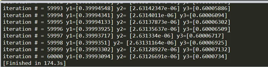
• 1. Case-1 (dt= 0.01)

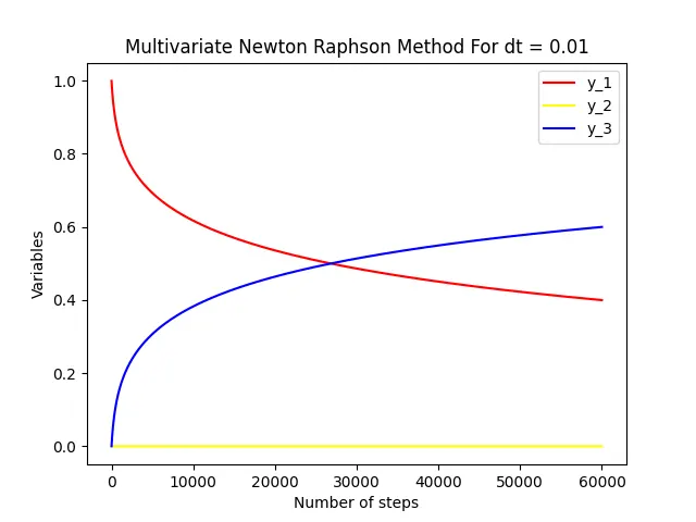
Figure(1)- Output graph for time step(dt) = 0.01

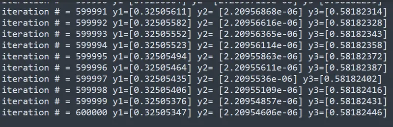
2. Case-2 (dt = 0.001)

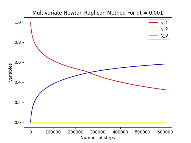
Figure(2)- Output graph for time step(dt) = 0.001

3. Case-3 ( dt =0.1)

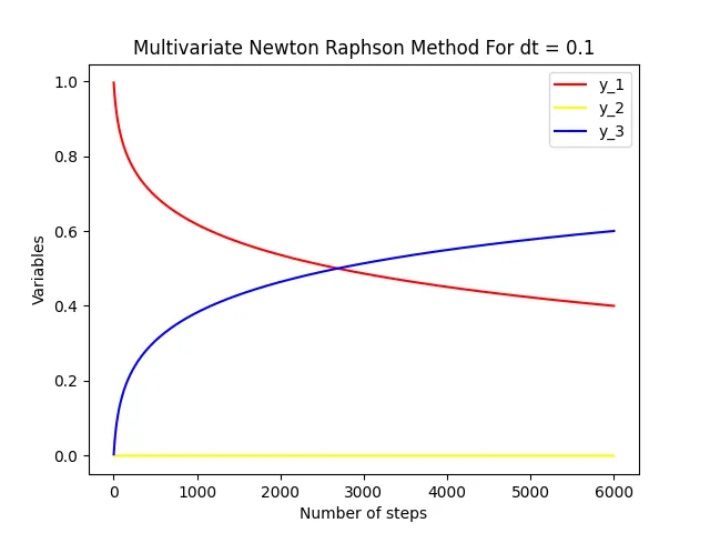
Figure(3)- Output graph for time step(dt) = 0.1

Selecting an appropriate time step size:-

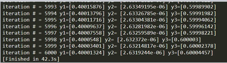
Before running the code and obtaining a solution, the time step dt is first set to 0.01. Run the simulation a second time with the time step value set to 0.001. However, the plot and solution are identical. The simulation was run a third time with the time step aggressively raised to dt =0.1. But nothing has changed as of yet. The length of the simulation also didn't vary significantly. This means that the change in time step does not affect the solution, which is stable and finally converges to produce fully meaningful findings. Therefore, the simulation is unaffected by the time step size. Since we are employing the implicit technique as an iterative solver and it is unaffected by the time step size, the simulation is stable.

If we utilize an explicit method as the iterative solver, the change in time step size can have an impact on the solution. Despite being relatively challenging to implement, implicit techniques can perform incredibly well in complex scenarios like the stiffness of non-linear coupled equations, rapid increases in temperature, pressure, and mass flow rate, etc. These situations can also occur when the implicit schemes are not easily codable.

Conclusion:-

The apex values of y1, y2, and y3 are changing fast concerning the time in the X-axis, as seen by the aforementioned graphs. As the solution advances in time, these variables are changing quickly. Due to the stiff nature of the equation system, this nature is observed.