Week 6 - Multivariate Newton Rhapson Solver

Objective: To solve the Set of equations given below using implicit Euler method/Backward differencing.

`dy_1/dt=-0.04y_1+10^4y_2y_3`

`dy_2/dt=0.04y_1-10^4y_2y_3-3*10^7y_2^2`

`dy_3/dt=3*10^1y_2^2`

Given data

Initial guesses for y

`y_1 = 1`

`y_2=0`

`y_3=0`

`alpha=1`

`time=10 text( minute)`

Theory

From the above set of differential equations, we can see that there are three independent variables and these kinds of problems are termed as coupled in nature. in order to solve this kind of coupled problem we will use multivariate Newton Raphson technique.

The above differential equation can be written as:

`(y_1^n-y_1^(n-1))/(Deltat)=-0.04y_1^n+10^4y_2^ny_3^n`

`(y_2^n-y_2^(n-1))/(Deltat)=0.04y_1^n-10^4y_2^ny_3^n-3*10^7(y_2^n)^2`

`(y_3^n-y_3^n)/(Deltat)=3*10^7(y_2^n)^2`

By applying the Backward differencing method for teh abode ODE's corresponding equations are obtained:

`f_1^n=y_1^n+Deltat(0.04y_1^n-10^4y_2^ny_3^n)-y_1^n=0`

`f_2^n=y_2^n+Deltat(0.04y_1^n-10^4y_2^ny_3^n-3*10^7(y_2^n)^2)-y_2^(n-1)=0`

`f_3^n=y_3^n+Deltat(3*10^7(y_2^n)^2)-y_3^(n-1)=0`

where,3

`y_n=y^text(new)`

`y^(n-1)=y^text(old)`

Then we will be computing the Jacobian matrix.

`J=[[(delf_1^n)/(dely_1^n),(delf_1^n)/(dely_2^n),(delf_1^n)/(dely_3^n)],[(delf_2^n)/(dely_1^n),(delf_2^n)/(dely_2^n),(delf_2^n)/(dely_3^n)],[(delf_3^n)/(dely_1^n),(delf_3^n)/(dely_2^n),(delf_3^n)/(dely_3^n)]]`

Now we will use a general equation of the multivariate Newton Raphson:

`y^text(new)=y^text(old)-alpha*J^-1*F`

Where,

`y^text(new)` is the new iteration value obtained with respect to initial guess value.

y^text(old)` is the value obtained from the previous iteration.

`alpha` is a relaxation factor.

`J^-1` is the inverse of jacobian matrix consisting of derivative of coupled equation.

F is the matrix containing the given system of equations.

`F=[[f_1],[f_2],[f_3]]`

Code with Explanation

"""
program to solve the system of coupled equations

dy1/dt=-0.04*y1+10^y2y3
dy2/dt= 0.04*y1-10^4y2y3-3*10^7(y2)^2
dy3/dt = 3*10^7(y2)^2


using newton raphson multivariate method
"""


import numpy as np
from numpy.linalg import inv
import matplotlib.pyplot as plt

def f1(y1, y2, y3,y_old1,y_old2,y_old3,dt):

	"""
	First Non linear equation
	"""
	return (y_old1 + h*(-0.04*y1 + (pow(10,4)*y2*y3)) - y1)

def f2(y1, y2, y3,y_old1,y_old2,y_old3,dt):
	"""
	Second non linear equation 
	"""
	return(y_old2 + h*(0.04*y1 - (pow(10,4)*y2*y3) - (3*pow(10,7)*pow(y2,2))) - y2)

def f3(y1, y2, y3,y_old1,y_old2,y_old3,dt):
	"""
	Third non linear equation 
	"""
	return(y_old3 + h*(3*pow(10,7)*pow(y2,2)) - y3)

def jacobian(y1, y2, y3,y_old1,y_old2,y_old3,h):
	"""
	Defining Jacobian
	"""

	j = np.zeros((3,3))			#3X3 Zero matrix
	dy = 1e-10   				# step size   


	# Row 1
	j[0,0] = (f1(y1+dy,y2,y3,y_old1,y_old2,y_old3,h)-f1(y1,y2,y3,y_old1,y_old2,y_old3,h))/dy;
	j[0,1] = (f1(y1,y2+dy,y3,y_old1,y_old2,y_old3,h)-f1(y1,y2,y3,y_old1,y_old2,y_old3,h))/dy;
	j[0,2] = (f1(y1,y2,y3+dy,y_old1,y_old2,y_old3,h)-f1(y1,y2,y3,y_old1,y_old2,y_old3,h))/dy;

	# Row 2
	j[1,0] = (f2(y1+dy,y2,y3,y_old1,y_old2,y_old3,h)-f2(y1,y2,y3,y_old1,y_old2,y_old3,h))/dy;
	j[1,1] = (f2(y1,y2+dy,y3,y_old1,y_old2,y_old3,h)-f2(y1,y2,y3,y_old1,y_old2,y_old3,h))/dy;
	j[1,2] = (f2(y1,y2,y3+dy,y_old1,y_old2,y_old3,h)-f2(y1,y2,y3,y_old1,y_old2,y_old3,h))/dy;

	#Row 3
	j[2,0] = (f3(y1+dy,y2,y3,y_old1,y_old2,y_old3,h)-f3(y1,y2,y3,y_old1,y_old2,y_old3,h))/dy;
	j[2,1] = (f3(y1,y2+dy,y3,y_old1,y_old2,y_old3,h)-f3(y1,y2,y3,y_old1,y_old2,y_old3,h))/dy;
	j[2,2] = (f3(y1,y2,y3+dy,y_old1,y_old2,y_old3,h)-f3(y1,y2,y3,y_old1,y_old2,y_old3,h))/dy;

	return j     


# defining initial guess
y_old = np.zeros((3,1))				#column vector
y_old[0] = 1
f = np.zeros((3,1)) 				#column vector
y_new = np.zeros((3,1)) 			#column vector
alpha = 1 #relaxation factor
tol = 1e-10
h = 0.1    							# Time step size
t = np.arange(0,600,h)

y_1 = []
y_2 = []
y_3 = []

# Starting Newton Raphson Loop

for i in range(0,len(t)):
	y_guess = np.copy(y_old)

	error = 9e9
	while error > tol:
		j = jacobian(y_new[0],y_new[1],y_new[2],y_old[0],y_old[1],y_old[2],h);
		f[0] = f1(y_guess[0],y_guess[1],y_guess[2],y_old[0],y_old[1],y_old[2],h);
		f[1] = f2(y_guess[0],y_guess[1],y_guess[2],y_old[0],y_old[1],y_old[2],h);
		f[2] = f3(y_guess[0],y_guess[1],y_guess[2],y_old[0],y_old[1],y_old[2],h);
		y_new = y_guess-alpha*np.matmul(inv(j),f)
		error = max(abs(y_new-y_guess))
		y_guess = y_new

	y_old = y_new
	y_1.append(y_new[0])
	y_2.append(y_new[1])
	y_3.append(y_new[2])

#plotting
plt.figure(1)
plt.plot(t,y_1,label='y1')
plt.plot(t,y_2,label='y2')
plt.plot(t,y_3,label='y3')
plt.xlabel('Time')
plt.ylabel('variables(species)')
plt.legend(['y_1','y_2','y_3'])
plt.title('multivariate Newton raphson')
plt.legend()
plt.show()

Plots

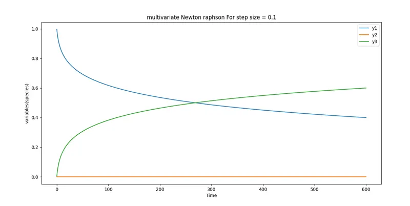
Case 1: Step size = 0.1

Conclusion

From the Above graphs we can see that the approximate values of `y_1` and `y_3` are changing continuously with respect to time. for the value of `y_` we cannot observe the change because the value of `y_2` is really small which is not shown in the scale of above graph. these values change rapidly as the solution marches forward in time.

The value of time step we used in the above case was 0.1 but changing the values of the timestep will not affect the result very much. The reason for this is we are using a implicit scheme. The only issue we will be facing while changing the timestep would be the computational time.