Week 6 - Multivariate Newton Rhapson Solver

Multivariate Newton Rhapson Solver

OBJECTIVE:

The main objective of this challenge is to solve a set of stiff ODE's by using Multivariate Newton Raphson method by writing code in python. The set of equations is solved by using Implicit euler method/ backward differencing method.

The set of equations to be solved are:

`(dy_1/dt) = -0.04*y_1 + 10^4*y_2*y_3`

`(dy_2/dt) = 0.04*y_1-10^4*y_2*y_3-3.10^7*y_2^2`

`(dy_3/dt) = 3.10^7*y_2^2`

By looking the above equations, it is clear that the equations are coupled which has to be solved all at a once. To do so we are using Multivariate Newton's Raphson method to find the roots. Newton Raphson Methos is a iterative technique used to solve the roots of a non -linear equations.

`Y^( New) = Y^(old ) - alpha*J^(-1)*F`

Here,

Y new = New values for Y after each iteration

Y_old = Initial guess values for Y to start the iteration

alpha = Relaxation factor

J^-1 = Jacobian matrix (m x n) which gives us the all possible derivatives for each variable in each function.

Where,

m = Rows of the matrix indicates the function

n = Columns of the matrix indicates the derivaties of each dependant variable

F = function matrix

As per the challange given, Jacobian matrix has to find numerically which is defined as below:

`Y^(New) = [(y_1^(New)),(y_2^(New)),(y_3^(New))]`

`Y^(old) = [(y_1^(old)),(y_2^(old)),(y_3^(old))]`

`J = [((df_1)/dy_1, (df_1)/dy_2,(df_1)/dy_3),((df_2)/dy_1,(df_2)/dy_2,(df_2)/dy_3),((df_3)/dy_1,(df_3)/dy_2,(df_3)/dy_3)]`

To convert the above differential equations into non linear equations, we are using backward differencing method which is also called as Implicit Euler method.

`f^'(x_i) = (f(x_i) - f(x_(i-1)))/(deltax)`

`dy/dt = f(y_i)`

`(y_i^n - y_i^(n-1))/(deltat) = f(y_i)`

`y_i^(n-1) +f(y_i)*deltat -y_i^n = 0`

The above set of equations at time step n = 1,

`f1 = y_1^0 + (-0.04*y_1 + 10^4*y_2*y_3)*(deltat) - y_1^1`

`f_2 = y_2^0 +(0.04*y_1 - 10^4*y_2*y_3 - 3.10^7*y_2^2)*deltat - y_2^1`

`f_3 = y_3^0+(3.10^7*y_2^2)*delt-y_3^1`

Similar to the above way, we will iterate the system for 10 minutes with various time steps to find the roots of the equations. The initial guesses for the y values are given as y1 = 1, y2 = 0, y3 = 0.

CODE SNIPPET:

"""
	Study of Multivariate Newton Raphson Method by using some set of equations
	The Simulation has to run for 10 mins which is 600 secs
	After the simulating with various time steps, Understanding the importance of time step.

	Set of Equations:

	dy1/dt = -0.04*y1 + 10^4*y2*y3
	dy2/dt = 0.04*y1-10^4*y2y3 - 3.10^7*y2^2
	dy3/dt = 3.10^7*y2^2

	Using Implicit euler method/Backward differencing mathod to find the roots

"""
import numpy as np
from numpy.linalg import inv
import matplotlib.pyplot as plt

#Defining the functions

def f1(y1_old,y1,y2,y3,dt):
	return (y1_old + dt*(-0.04*y1 + y2*y3*1e4) - y1)

def f2(y2_old,y1,y2,y3,dt):
	return (y2_old + dt*(0.04*y1 - (1e4*y2*y3) -(3e7*y2*y2)) -y2)

def f3(y3_old,y1,y2,y3,dt):
	return (y3_old + dt*(3e7*y2*y2) - y3)

# defining jacobian matrix which gives possible derivative for each term
def jacobian(y1_old,y2_old,y3_old,y1,y2,y3,dt):
	
	#Creating 3x3 matrix because we have 3 functions and 3 dependant variables
	J = np.ones((3,3))
	#step size
	dy = 1e-6 
	# Row 1
	J[0,0] = (f1(y1_old,y1+dy,y2,y3,dt)-f1(y1_old,y1,y2,y3,dt))/dy
	J[0,1] = (f1(y1_old,y1,y2+dy,y3,dt)-f1(y1_old,y1,y2,y3,dt))/dy
	J[0,2] = (f1(y1_old,y1,y2,y3+dy,dt)-f1(y1_old,y1,y2,y3,dt))/dy
	 # Row 2
	J[1,0] = (f2(y2_old,y1+dy,y2,y3,dt)-f2(y2_old,y1,y2,y3,dt))/dy
	J[1,1] = (f2(y2_old,y1,y2+dy,y3,dt)-f2(y2_old,y1,y2,y3,dt))/dy
	J[1,2] = (f2(y2_old,y1,y2,y3+dy,dt)-f2(y2_old,y1,y2,y3,dt))/dy
	 # Row 3
	J[2,0] = (f3(y3_old,y1+dy,y2,y3,dt)-f3(y3_old,y1,y2,y3,dt))/dy
	J[2,1] = (f3(y3_old,y1,y2+dy,y3,dt)-f3(y3_old,y1,y2,y3,dt))/dy
	J[2,2] = (f3(y3_old,y1,y2,y3+dy,dt)-f3(y3_old,y1,y2,y3,dt))/dy
	
	return J

#Initial guess values for variables
y1_old = 1
y2_old = 0
y3_old = 0

#Creating a matrix for the guess values
Y_old = np.ones((3,1))
Y_old[0] = y1_old
Y_old[1] = y2_old
Y_old[2] = y3_old

#Creating a copy 
F = np.copy(Y_old)

#relaxation factor
alpha = 1
tol = 9e-6					
t = 600			#simulation time		
dt = 10		#time step
n = int(t/dt)	#number of time steps
#Creating a null array of dependant variables
x1 = []
x2 = []
x3 = []
iteration = []
#Starting the newton rapson loop
iter =1
for i in range(0,n):
	error = 9e9
	tol = 9e-6
	while error>tol:
		# Computing the Jacobian - old values are used
		J = jacobian(y1_old,y2_old,y3_old,Y_old[0], Y_old[1], Y_old[2],dt)
		# Computing the F vector - old values are used
		F[0] = f1(y1_old,Y_old[0],Y_old[1],Y_old[2],dt)
		F[1] = f2(y2_old,Y_old[0],Y_old[1],Y_old[2],dt)
		F[2] = f3(y3_old,Y_old[0],Y_old[1],Y_old[2],dt)
		# Computing the new values
		Y_new = Y_old - alpha*np.matmul(inv(J), F)
		# Computing the max abs error
		error = np.max(np.abs(Y_new-Y_old))
		print(error)
		#Updating the old values
		Y_old = Y_new
	#log message
	log_message = 'iteration No. = {0} y1 = {1} y2 = {2} y3 = {3}'.format(iter,Y_new[0],Y_new[1],Y_new[2])
	print(log_message)
	# Storing the values for plotting
	x1.append(Y_new[0])
	x2.append(Y_new[1])
	x3.append(Y_new[2])
	iter = iter+1
	iteration.append(iter)
	Y_old = Y_new
        # Upadting the y_old values for next iteration
	y1_old = Y_new[0]
	y2_old = Y_new[1]
	y3_old = Y_new[2]
	error = 9e9


#plotting the variables
plt.plot(iteration, x1)
plt.plot(iteration, x2)
plt.plot(iteration, x3)
plt.xlabel('Simulation time')
plt.ylabel('Variable Value')
plt.grid('on')
plt.legend(['y1','y2','y3'])
plt.title('Multivariate Newton Raphson method for time step size of 10s')
plt.show()

PROCEDURE:

• Before writing the code importing the essential libraries to do the simulation.
• Defining the function as mentioned in the thoery.
• Defining the Jacobian matrix and solving the function numerically by each variable as per theory.
• Defining initial guess values for y.
• Creating a Y_old matrix and using the initial guess as fuction.
• Definig all the time related data as per challenge simulation time to be 10 mins which is 600secs with suitable time step.
• Starting the Newton Raphson method with outer time loop by assembling the ODE system inside a while loop.
• Running the while loop till convergence and updating the y_old values for next iteration.
• Obtaining the new values by using appending method.
• Plotting the results.

RESULTS:

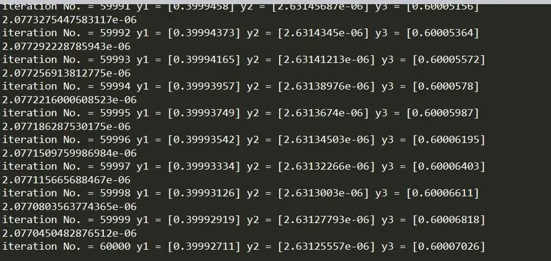
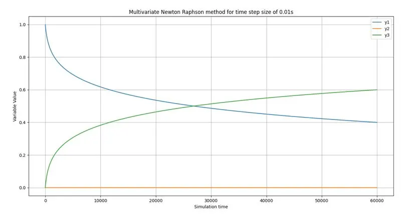
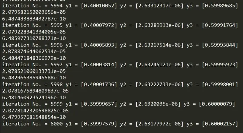
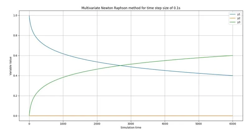
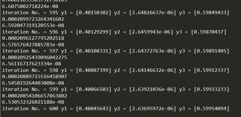
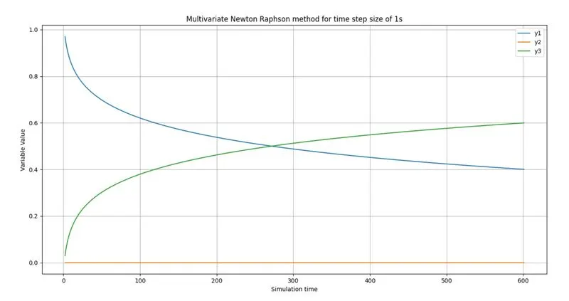
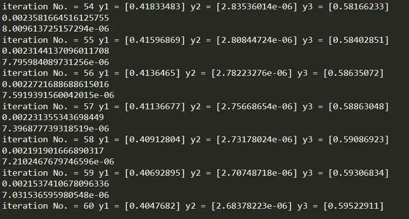
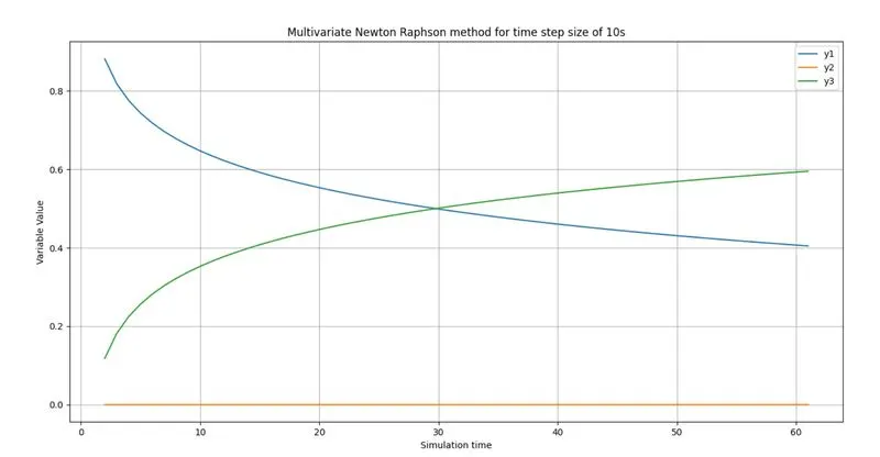
What is the ideal time step?

Before deciding the ideal time step, we know as per the previous challenges the time step won't affect the simulation runs at Implict condition. But the thing I observed from the above plots that even though the results are obatained which is alomst similar, the accuracy which is important thing is varying by increasing the time step value ( This can be observed from the plots and results of time step of 1s and 10s). If the accuracy is the prime factor for your simuation, run with smaller time steps which takes time to complete the simulation. In this simulation, the values of time steps 0.01s and 0.1s are varying but not too much. By keeping simulation time and accuracy in mind, the time step of 0.1s is suitable for this challenge.