Week 6 - Multivariate Newton Rhapson Solver

AIM:

       To solve the system of ODE using Newton Raphson method.

GIVEN:

`(dy_1)/dt= -0.04y_1+10^4 y_2 y_3`

`(dy_2)/dt=0.04y_1-10^4 y_2 y_3- 3.10^7 y_2^2`

`(dy_3)/dt=3.10^7 y_2^2`

Since the given ODEs are stiff ODE, the implicit method is used to solve stiff ODE. The backward differentiation is used to solve the ODE using implicit method.

`f^' (x_i )= (f(x_i )-f(x_(i-1)))/(triangle x)`

`trianglex` = step size

NEWTON RAPHSON METHOD:

Newton Raphson method, is a root finding algorithm which produces successively better approximation to the roots of a real-valued function. The most basic version starts with a single variable function f defined for a real variable x, the function’s derivative f’, and a initial guess x0 for a root of f. if the function satisifies sufficient assumptions and the initial guess is close, then

`X_(n+1) = x_n – f(x_n)/ (f’(x_n )`

MULTIVARIATE NEWTON RAPHSON METHOD:

Multivariate newton Raphson method used to solve stiff systems of coupled equations to find the roots. The formula for multivariate newton Raphson method is

`Y_(New) = y_(old) – alpha.J^(-1).F`

Where, y_new is new value that is updated after every iteration.

               Y_old is the old value

               Alpha is the relaxation factor

               J is jacobian matrix

               F is function matrix

Jacobian matrix is calculated numerically by finding the partial derivatives for every function with every variable and arrange it in a matrix form

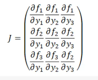
Here f_1, f_2, f_3 are the functions of ODE

`f_1=y_1^(old) +h*(-0.04y_1+10^4 y_2 y_3 )-y_1`

`f_2=y_2^(old)+h*(0.04y_1-10^4 y_2 y_3-3.10^7 y_2^2 )-y_2`

`f_3=y_3^old+h*(3.10^7 y_2^2 )-y_3`

By substituting all the above equation in multivariate newton Raphson,

 

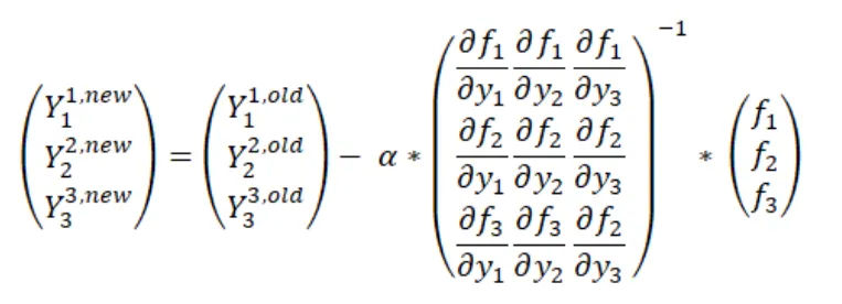
The initial conditions y_1^old,y_2^old and y_3^old are assumed as 1,0,0 and simulation is done for 10 minutes.

CODING APPROACH:

• The required modules are imported in python.
• The three given functions are defined. Then the jacobian matrix is defined.
• The jacobian matrix is solved by using numerical method.
• Then the simulation time and step size is defined.
• The outer time loop is defined.
• Running the newton Raphson solver till convergence.
• Obtain the new values and update them.
• The loop is ended.
• Then the plotting is made between iterations and Y.

PYTHON CODE:

"""
	PROGRAM TO CALCULATE SYSTEM OF COUPLED NON LINEAR EQUATIONS
	(dy_1)/dt= -0.04y_1+10^4 y_2 y_3
    (dy_2)/dt=0.04y_1-10^4 y_2 y_3-〖3.10〗^7 y_2^2
    (dy_3)/dt=〖3.10〗^7 y_2^2

"""

import numpy as np
from numpy.linalg import inv
import matplotlib.pyplot as plt

def f1(y1_old,y1_new,y2_new,y3_new,h):
	"""
		First Non Linear Equation
	"""
	return y1_old + h*(-0.04*y1_new + pow(10,4)*y2_new*y3_new) - y1_new

def f2(y2_old,y1_new,y2_new,y3_new,h):
	"""
		Second Non Linear Equation
	"""
	return y2_old + h*(0.04*y1_new - pow(10,4)*y2_new*y3_new - 3*pow(10,7)*pow(y2_new,2)) - y2_new

def f3(y3_old,y1_new,y2_new,y3_new,h):
	"""
		Third Non Linear Equation
	"""
	return y3_old + h*(3*pow(10,7)*pow(y2_new,2)) - y3_new

def jacobian(y1_old,y2_old,y3_old,y1_new,y2_new,y3_new,h):
	"""
		defining the jacobian matrix
	"""

	J = np.ones((3,3))

	#step size
	dy = 1e-6

	#creating the matrix
	#Row 1
	J[0,0] = (f1(y1_old,y1_new+dy,y2_new,y3_new,h) -  f1(y1_old,y1_new,y2_new,y3_new,h))/dy
	J[0,1] = (f1(y1_old,y1_new,y2_new+dy,y3_new,h) -  f1(y1_old,y1_new,y2_new,y3_new,h))/dy
	J[0,2] = (f1(y1_old,y1_new,y2_new,y3_new+dy,h) -  f1(y1_old,y1_new,y2_new,y3_new,h))/dy

	#ROW 2
	J[1,0] = (f2(y1_old,y1_new+dy,y2_new,y3_new,h) -  f2(y1_old,y1_new,y2_new,y3_new,h))/dy
	J[1,1] = (f2(y1_old,y1_new,y2_new+dy,y3_new,h) -  f2(y1_old,y1_new,y2_new,y3_new,h))/dy
	J[1,2] = (f2(y1_old,y1_new,y2_new,y3_new+dy,h) -  f2(y1_old,y1_new,y2_new,y3_new,h))/dy

	#ROW 3
	J[2,0] = (f3(y1_old,y1_new+dy,y2_new,y3_new,h) -  f3(y1_old,y1_new,y2_new,y3_new,h))/dy
	J[2,1] = (f3(y1_old,y1_new,y2_new+dy,y3_new,h) -  f3(y1_old,y1_new,y2_new,y3_new,h))/dy
	J[2,2] = (f3(y1_old,y1_new,y2_new,y3_new+dy,h) -  f3(y1_old,y1_new,y2_new,y3_new,h))/dy


	return J

# INITIAL GUESS VALUES
y1_old = 1
y2_old = 0
y3_old = 0


error = 1e9

# CREATING THE COLUMN VECTOR
Y_old = np.ones((3,1))
Y_old[0] = y1_old
Y_old[1] = y2_old
Y_old[2] = y3_old


F = np.copy(Y_old)

iterations = [] 
Y_1 = []
Y_2 = []
Y_3 = []

# DEFINING THE NR PARAMETERS
alpha = 1
tol = 1e-12
t_start = 0
t_end = 600
n = 60000
h = (t_end -t_start)/(n-1)
t = np.arange(t_start,t_end,h)

iter = 1
for i in range(0,len(t)):
	while error > tol:
		# COMPUTING THE JACOBIAN
		J = jacobian(y1_old,y2_old,y3_old,Y_old[0],Y_old[1],Y_old[2],h)

		#COMPUTING THE F VECTOR
		F[0] = f1(y1_old,Y_old[0],Y_old[1],Y_old[2],h)
		F[1] = f2(y2_old,Y_old[0],Y_old[1],Y_old[2],h)
		F[2] = f3(y3_old,Y_old[0],Y_old[1],Y_old[2],h)

		# COMPUTING NEW VALUES
		Y_new = Y_old - alpha*(np.matmul(inv(J),F))

		#COMPUTING THE ERROR
		error = np.max(np.abs(Y_new-Y_old))
		print(error)

		#UPDATING THE NEW VALUES
		Y_old = Y_new

		log_message = 'iteration # = {0} y1 = {1} y2 = {2} y3 = {3}'.format(iter,Y_new[0],Y_new[1],Y_new[2])
		print(log_message)
		
		iterations.append(iter)
		Y_1.append(Y_new[0])
		Y_2.append(Y_new[1])
		Y_3.append(Y_new[2])

	iter = iter+1
	error = 1e9
	Y_old = Y_new
	y1_old = Y_new[0]
	y2_old = Y_new[1]
	y3_old = Y_new[2]

#PLOTTING
plt.plot(iterations,Y_1,color='red')
plt.plot(iterations,Y_2,color='blue')
plt.plot(iterations,Y_3,color='green')
plt.grid('on')
plt.xlabel('time (sec)')
plt.ylabel('Y')
plt.title('variation of Y with time dt ='+str(h))
plt.legend(['y1','y2','y3'])
plt.show()

RESULT:

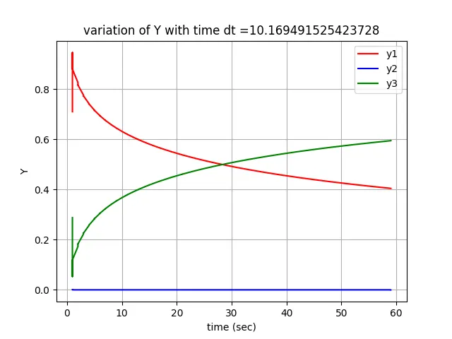
FOR dt = 10:

 

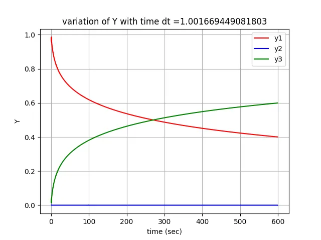
FOR dt = 1

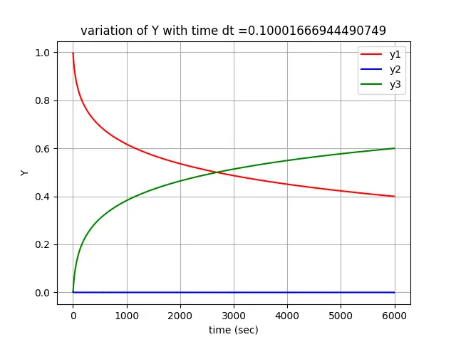
FOR dt = 0.1

FOR dt = 0.01

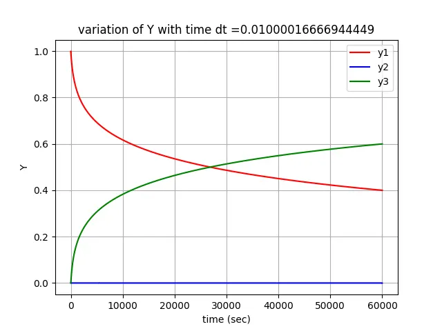
From the plots we can observe that when we increase the dt the solution keeps on changing and remains constant after reaching dt = 0.1. so the optimal step size is 0.1.

There is not much change in graph as we are using the implicit method but if we used the explicit method the graph might be changed.From this we can say that implicit method doesnot have any effect of time step.