Week 6 - Multivariate Newton Rhapson Solver

AIM:

Solve the given set of equations using Implicit Euler Method/Backward Differencing, incorporating numerical jacobian. For this, it is expected that we assume the initial conditions as:

`y_1`=1, `y_2`=0, `y_3`=0

We have are expected to run the simulation for 10 minutes and select an appropriate step size and mention the reasoning it as well.

THEORY:

Here, in this assignment, we will be solving the given ODE system to figure out the values for `y_1`,`y_2` and `y_3`. The initial guess values for these 3 variable provided along with the ODE system. Now, by employing the Backward Differencing method to the ODE system, they can be represented in the following manner:

`f_1=y_1^(n-1)+h(-0.04y_1^n+10^4y_2^ny_3^n)-y_1^n=0`

`f_2=y_2^(n-1)+h(0.04y_1-10^4y_2y_3-3*10^7y_2^2)-y_2^n=0`

`f_3=y_2^(n-1)+h(3*10^7y_2^2)-y_3^n=0`

Here, 'h' represents the time-step.

This above system of equations in nothing but a system of non-linear equations. These have to be solved for each of the time steps. For example, for n=1, we have:

`f_1=y_1^0+h(-0.04y_1+10^4y_2y_3)-y_1=0`

`f_2=y_2^0+h(0.04y_1-10^4y_2y_3-3*10^7y_2^2)-y_2=0`

`f_3=y_2^0+h(3*10^7y_2^2)-y_3=0`

And now,

`F=[[f_1],[f_2],[f_3]]`

As we know, `Y_(1,guess)=1,Y_(2,guess)=0 and Y_(3,guess)=0`;

`Y_(Guess)=[[Y_(1,guess)],[Y_(2,guess)],[Y_(3,guess)]]`

Here, we use an iterative method such as Newton Rhapson Technique and as it is a stiff system,we use Implicit Integration Scheme/Backward Difference Scheme.

`Y^("new")=Y^("old")-alpha(J^(-1))*F`

where, `alpha ->`relaxation factor

and J`->`is the Jacobian Matrix.

This Jacobian Matrix is written as,

`J=[[(partialf_1)/(partialy_1),(delf_1)/(dely_2),(delf_1)/(dely_3)],[(delf_2)/(dely_1),(delf_2)/(dely_2),(delf_2)/(dely_3)],[(delf_3)/(dely_1),(delf_3)/(dely_2),(delf_3)/(dely_3)]]`

Now the following code to employed to compute the ODE system for `y_1,y_2 and y_3`

CODE:

https://drive.google.com/file/d/1hLGSVf_7W_2xW2wA4rzXK6hGr14788CK/view?usp=sharing

RESULTS:

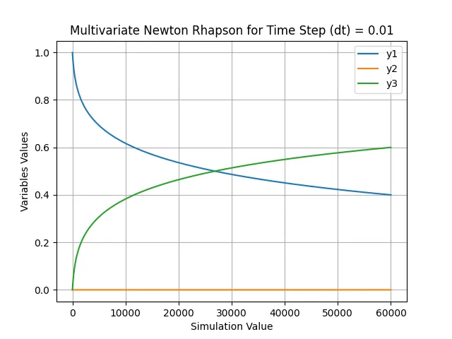
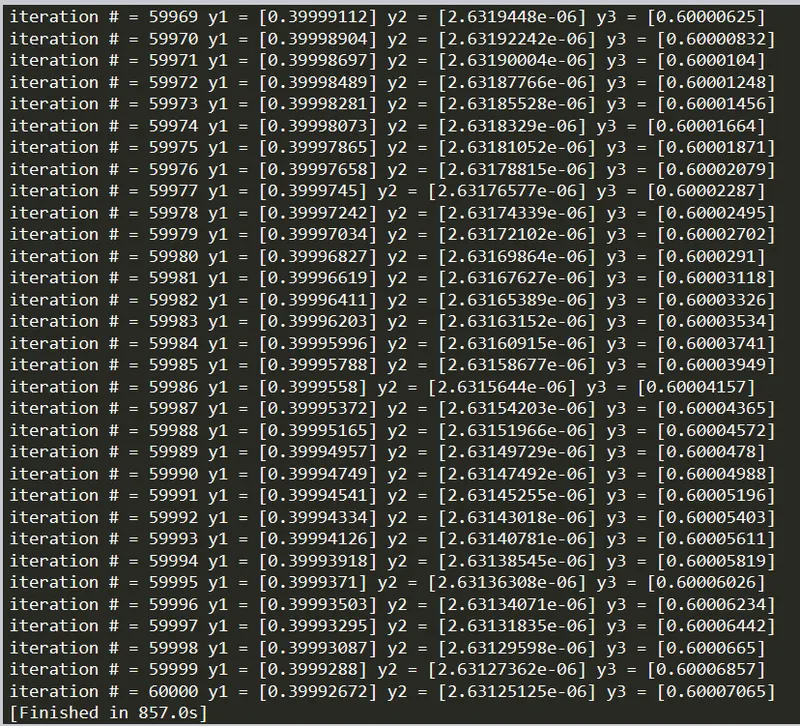
Time Step = 0.01 and n = 60000

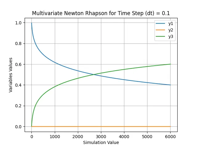
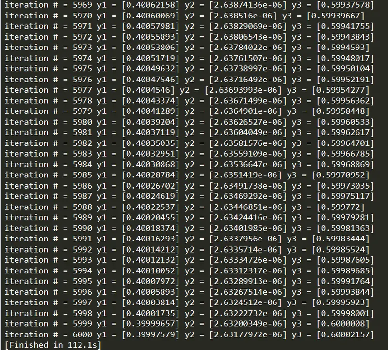
Time step = 0.1 and n = 6000

Time Step = 1 and n = 600

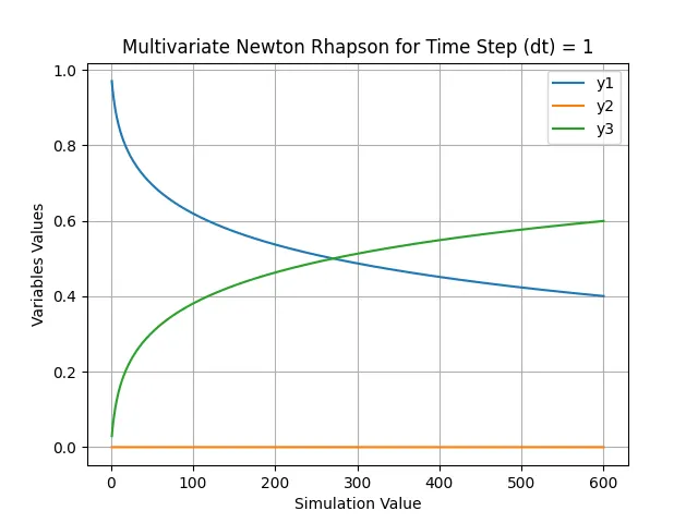
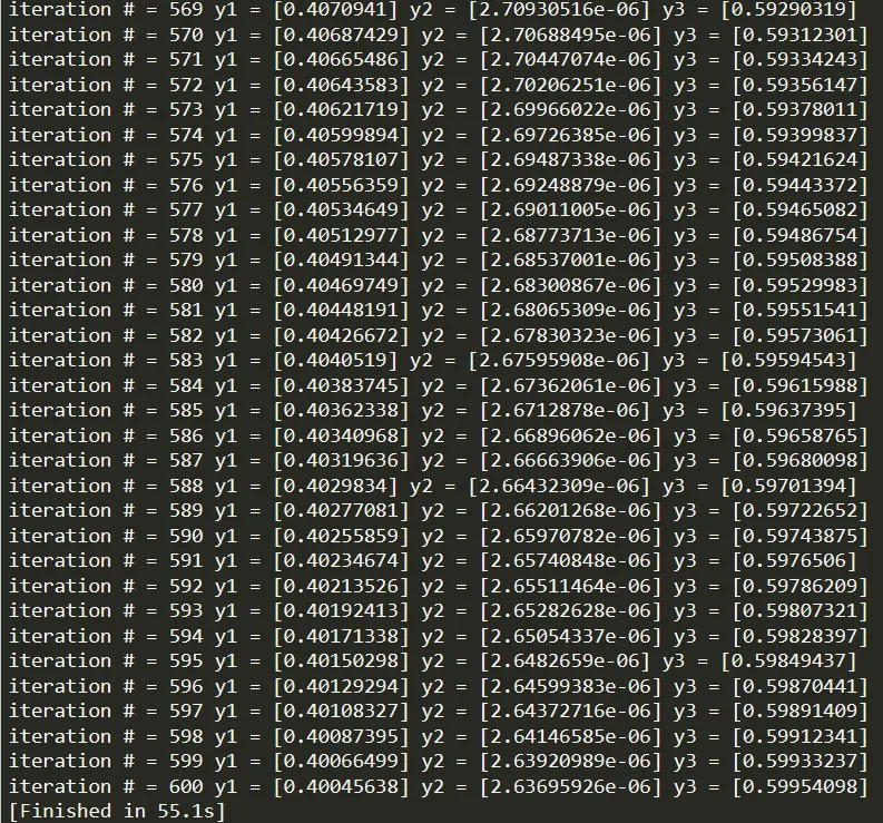
From the results and the obtained graphs, it can be seen that there is a considerable amount of change in the values of y1 and y3 and keeps on varying further with time. Meanwhile, y2 doesn't seem to vary as much and remains mostly constant. This shows the stiff characteristic of the ODE system. As seen from the results, for time steps 0.1 and 0.01, the values of the variable remain almost constant. From a cost and resourse saving perspective, it would be wise to opt for 0.1 time step as this more optimum as compared to 0.01 time step.