Week 6 - Multivariate Newton Rhapson Solver

AIM: To solve the given set ofcoupled non-linear equations by using Implicit Euler Method/ Backward Differencing.

Introduction:

In numerical analysis, Newton's method, also known as the Newton–Raphson method is a root-finding algorithm which produces successively better approximations to the roots (or zeroes) of a real-valued function.

Newton’s method uses first and second derivatives and indeed performs better.

Given a starting point, construct a quadratic approximation to the objective function that matches the first and second derivative values at that point. We then minimize the approximate (quadratic function) instead of the original objective function. The minimizer of the approximate function is used as the starting point in the next step and repeat the procedure iteratively.

Solution:

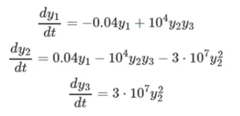
We have,

dy1/dt = -0.04*y1 + 10^4*y2*y3
dy2/dt = 0.04*y1 -10^4*y2*y3 - 3*10^7*y2*y2
dy3/dt = 3*10^7*y2*y2

Initial Conditions:

y1o = 1

y2o = 0

y3o = 0



By using Implicit Euler Method/ Backward Differencing the above equations can be written as

(y1^(n) - y1^(n-1))/delta(t) = -0.04*y1 + 10^4*y2*y3                         => f1

(y2^(n) - y2^(n-1))/delta(t) = 0.04*y1 -10^4*y2*y3 - 3*10^7*y2*y2            => f2

(y3^(n) - y3^(n-1))/delta(t) = 3*10^7*y2*y2                                  => f3



f1^(n) = y1^(n) + delta(t)*(0.04*y1^(n) - 10^4*y2^(n)*y3^(n)) - y1^(n-1) = 0

f2^(n) = y2^(n) + delta(t)*(0.04*y1^(n) - 10^4*y2^(n)*y3^(n) - 3.10^(7)*(y2^(n))^2) - y1^(n-1)=0

f3^(n) = y3^(n) + delta(t)*(3*10^(7)*(y2^(n))^2) - y3^(n-1) = 0

where,

yn = yNew

y(n-1) = yOld



Therefore, F =        [ f1                Y_guess = [ y1,guess

                        f2                            y2,guess

                        f3]                           y3,guess] 



Y_New = Y_guess - alpha*J^(-1)*F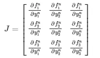

Python Code:

"""
Program to solve the system of
coupled non-linear equations

dy1/dt = -0.04*y1 + 10^4*y2*y3
dy2/dt = 0.04*y1 -10^4*y2*y3 - 3*10^7*y2*y2
dy3/dt = 3*10^7*y2*y2

Modules required
1. numpy is required for matrix multiplication
2. inv is required for computing the inverse of a matrix


"""
import numpy as np
from numpy.linalg import inv
import matplotlib.pyplot as plt

def f1(y1_old, y1, y2, y3, dt):
	"""
	First non-linear equation
	"""
	return (y1_old + dt*(-0.04*y1 + y2*y3*pow(10,4)) - y1)

def f2(y2_old, y1, y2, y3, dt):
	"""
	Second non-linear equation
	"""
	return (y2_old + dt*(0.04*y1 - (pow(10,4)*y2*y3) - (3*pow(10,7)*pow(y2,2))) - y2)

def f3(y3_old, y1, y2, y3, dt):
	"""
	Third non-linear equation
	"""
	return (y3_old + dt*(3*pow(10,7)*pow(y2,2)) - y3)

def jacobian(y1_old, y2_old, y3_old, y1, y2, y3, dt):
	"""
	Defining the Jacobian
	"""
	# 3 by 3 unit matrix
	J = np.ones((3,3))

	h = 1e-5

	# Row 1
	J[0,0] = (f1(y1_old,y1+h,y2,y3,dt) - f1(y1_old,y1,y2,y3,dt))/h
	J[0,1] = (f1(y1_old,y1,y2+h,y3,dt) - f1(y1_old,y1,y2,y3,dt))/h
	J[0,2] = (f1(y1_old,y1,y2,y3+h,dt) - f1(y1_old,y1,y2,y3,dt))/h

	# Row 2
	J[1,0] = (f2(y2_old,y1+h,y2,y3,dt) - f2(y2_old,y1,y2,y3,dt))/h
	J[1,1] = (f2(y2_old,y1,y2+h,y3,dt) - f2(y2_old,y1,y2,y3,dt))/h
	J[1,2] = (f2(y2_old,y1,y2,y3+h,dt) - f2(y2_old,y1,y2,y3,dt))/h

	# Row 3
	J[2,0] = (f3(y3_old,y1+h,y2,y3,dt) - f3(y3_old,y1,y2,y3,dt))/h
	J[2,1] = (f3(y3_old,y1,y2+h,y3,dt) - f3(y3_old,y1,y2,y3,dt))/h
	J[2,2] = (f3(y3_old,y1,y2,y3+h,dt) - f3(y3_old,y1,y2,y3,dt))/h

	return J

# Defining the initial guess values
y1_old = 1
y2_old = 0
y3_old = 0;

# initial error - Q: Will any value for error work?
error = 9e9

# numpy coloumn vector
Y_old = np.ones((3,1))
Y_old[0] = y1_old
Y_old[1] = y2_old
Y_old[2] = y3_old

# numpy column vector for F
F = np.copy(Y_old)

# Parameters for Newton Rhapson solver
alpha = 1
tol = 1e-6
t = 600
dt = 0.1
n = int(t/dt)
y_1 = []
y_2 = []
y_3 = []
iteration = []

# Starting the Newton Rhapson Loop
iter= 1

for i in range (0,n):

	while error > tol:
		# Computing the Jacobian - old values are used
		J = jacobian(y1_old, y2_old, y3_old, Y_old[0], Y_old[1], Y_old[2], dt)

		# Computing the F vector - old values are used
		F[0] = f1(y1_old, Y_old[0], Y_old[1], Y_old[2], dt)
		F[1] = f2(y2_old, Y_old[0], Y_old[1], Y_old[2], dt)
		F[2] = f3(y3_old, Y_old[0], Y_old[1], Y_old[2], dt)

		# Computing new values
		Y_new = Y_old - alpha*np.matmul(inv(J), F)

		# Computing max abs error
		error = np.max(np.abs(Y_new-Y_old))
		print(error,tol)

		# Updating old values - Q: Why is this important?
		Y_old = Y_new


	# log message
	log_message = 'iteration number = {0} y1 = {1} y2 = {2} y3 = {3}'.format(iter, Y_new[0], Y_new[1], Y_new[2])
	print(log_message)
	iter = iter+1

	y_1.append(Y_new[0])
	y_2.append(Y_new[1])
	y_3.append(Y_new[2])

	iteration.append(iter)
	Y_old = Y_new
	y1_old = Y_new[0]
	y2_old = Y_new[1]
	y3_old = Y_new[2]

	error = 9e9

# Plotting
plt.plot(iteration,y_1,color = 'r')
plt.plot(iteration,y_2,color = 'y')
plt.plot(iteration,y_3,color = 'b')
plt.xlabel('No. of Steps')
plt.ylabel('Species')
plt.legend(['y_1', 'y_2', 'y_3'])
plt.title('Multivariate Newton Rhapson Method for dt=0.1')
plt.show()

Results:

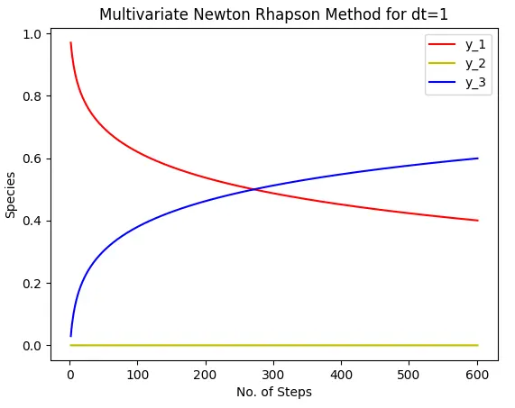
for dt = 1

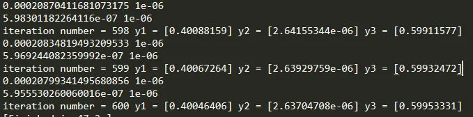
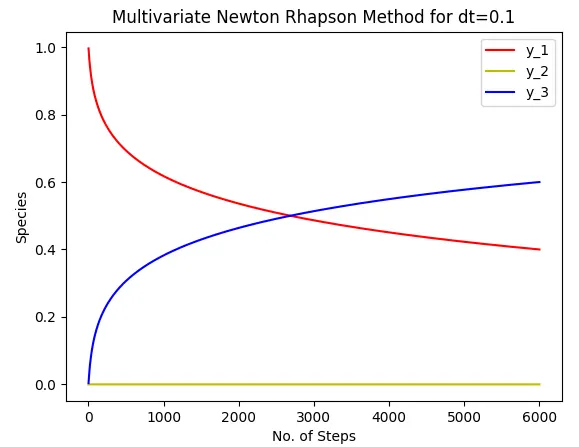
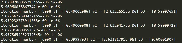
for dt = 0.1

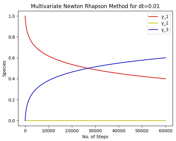
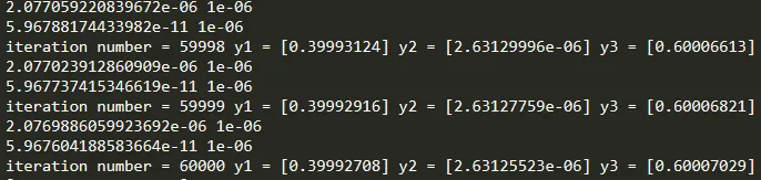
for dt = 0.01

Conclusion:

1. The valuess of y1, y2, y3 changes with respect to time. Due to small value of y2 the change in y2 values are very small.

2. The time step 0.1 is used. Even though the time step value varies like 1 and 0.01 the results are same.

We can conclude that 0.01 step size is suitable because the number of iterations are more so that accuracy is good.