Week 6: Conjugate Heat Transfer Simulation

Introduction

In this project we are required to setup a conjugate heat transfer flow through a pipe.The fluid flowing thorugh the pipe is air with a reynold's number of 7000 and the outer walls are being heated with a flux of -1000 W/m2.

Theory

Conjugate Heat Transfer

Conjugate Heat Transfer Analysis is used when there is heat transfer between 2 mediums mainly solid and fluids and where the heat transfer can occur in different modes.In solids the heat tranfser mode is mainly conduction while in fluids it is mainly through convection.

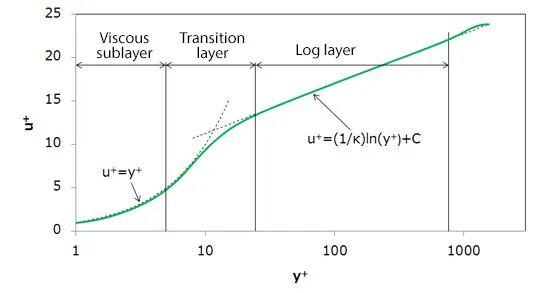
y+ and wall functions

In order to resolve flow near wall we can go for a finer mesh size but this increases the total computational time which is undesirable . Hence we use the wall funcations and y+.

Wall functions are used to model near wall velocity profiles at coarse grids and y+ is used to specify how fine or coarse our grids are.

ρ${\displaystyle \rho }$ - Density (kg/m3)

Ut${\displaystyle U_t}$- Shear Velocity (m/s)

μ${\displaystyle \mu }$ - Dynamic Viscosity (kg/m*s)

△y${\displaystyle △y}$- Mesh size (m)

The desirable range for y+ is y+ < 10(viscous sub layer) or 30<y+<500 (log law region). Using the y+ values obtained from post processing we can fine tune the mesh size for desired results.

Super Cycling

Since the time taken for fluids to converge is greater than the time taken for solids as a result we use a feature of converge called as super cycling where

1.Both the fluid and solid equations are solved with the transient solver.

2.After reaching the cycling stage time the transient solver is paused and the solid equations are solved using steady state solver and after reaching a steady state the transient solver is resumed and the process continues.

1.Geometry

A cylinder of Inner Radius = 0.015m and thickness = 0.005m is created using the cretae tool in converge.

1.2.Boundary Flagging

The different boundaries for the geometry are flagged.

Case Setup

1.1 Materials

The matrial is choosen to be air and solid simulation and reaction mechanism is checked since it is a CHT.

1.2 Solid Simulation

The outer wall for the cylinder is choosen to be Aluminium.

1.3 Reaction Mechanism

The elements and species for air is choosen.

2. Simulation Parameters

2.1 Run Parameters

The simulation is choosen to be a transient simulation

2.2 Simulation Time Parameters

The time parameters for the simulation is choosen as:

Start time = 0s , End Time = 0.5s , Time Step=1e-7

2.3 Solver Parameters

The solver scheme is choosen to be PISO and the type is choosen to be Density based.

3. Boundary Type

The important boundary conditions are:

1.Outer Wall : Temperature BC = -1000 W/m2

2.Sides:Velocity BC = Slip , Temperature BC (Newman BC)

3.Outlet:Pressure BC = 101325 Pa (Dirichlet BC)

4.Inlet: Velocity BC = 7.33 m/s (Dirichlet BC)

5.Interface : Fluid side = Velocity BC (Law of Wall) , Solid Side = Velocity BC (Dirichlet BC)

4.Regions and initialization

2 Regions are choosen 1.Fluid 2.Solid and are initialized with initial pressure and temperature.

5.Turbulence Model

The model is choosen to be RNG k-E

6. Super Cycling modelling

The below values are given for super cycling and coordinates inside the outer cylinder is choosen to monitor temperature values.

7.Base grid

The base grid is choosen to be 3 different values 0.002,.0.004,0.006 m .

8.Output files

The time interval for writting 3d ouput files is choosen as 0.005s (100 files).

THe time interval for writting text files is choosen as 0.001s (500 files)

Post Processing

The post processing of results is done using paraView software.

The base mesh size is influenced by 2 main factors 1.Grid independence and 2.y+ values

Grid Independence Test

The outlet temperature for the 3 different base mesh sizes is given

As the plot suggests for the 3 different base meh size the temperature converges to around 340 K.

Just by considering the grid independence test we can go with base mesh as 0.006m as the computation time is the least for this mesh but since this is a turbulent flow thorugh a pipe we should also conside the y+ values for the different mesh sizes

2. Y+

Y+ for 0.006m mesh

Y+ for 0.004m mesh size

Y+ for 0.002m mesh size

for both 0.006 and 0.004 the y+ values are in the buffer layer which is undesirable . For the 0.002m mesh the y+ values are in the viscous-sub layer range (y+ < 10) hence 0.002 can be choosen to be the apt mesh size.

1.0.002m base mesh

Grid

Velocity Distribution

Pressure Distribution

Effect of supercycling stage interval

We can observe , with the increase in supercycling stage the computation time decreases.