Week 6: Conjugate Heat Transfer Simulation

AIM: To setup a Conjugate Heat Transfer simulation through a cylindrical pipe.

Introduction:

The Conjugate Heat Transfer (CHT) analysis type allows for the simulation of heat transfer between solid and fluid domains by exchanging thermal energy at the interfaces between them.

The CHT approach has an advantage over FE thermal analyses in that wall heat transfer coefficients and their local variations on surfaces are directly calculated within the model rather than based on simplified empirical calculations. The CHT approach therefore has benefits for those applications where heat transfer is either non-uniform or difficult to calculate empirically.

Heat Transfer in a Solid:

In most cases, heat transfer in solids, if only due to conduction, is described by Fourier’s law defining the conductive heat flux, q, proportional to the temperature gradient: .

For a time-dependent problem, the temperature field in an immobile solid verifies the following form of the heat equation:

Heat Transfer in a Fluid:

Due to the fluid motion, three contributions to the heat equation are included:

The transport of fluid implies energy transport too, which appears in the heat equation as the convective contribution. Depending on the thermal properties on the fluid and on the flow regime, either the convective or the conductive heat transfer can dominate.

The viscous effects of the fluid flow produce fluid heating. This term is often neglected, nevertheless, its contribution is noticeable for fast flow in viscous fluids.

As soon as a fluid density is temperature-dependent, a pressure work term contributes to the heat equation. This accounts for the well-known effect that, for example, compressing air produces heat.

Accounting for these contributions, in addition to conduction, results in the following transient heat equation for the temperature field in a fluid:

Heat transfer in solids and heat transfer in fluids are combined in the majority of applications. This is because fluids flow around solids or between solid walls, and because solids are usually immersed in a fluid.

An accurate description of heat transfer modes, material properties, flow regimes, and geometrical configurations enables the analysis of temperature fields and heat transfer. Such a description is also the starting point for a numerical simulation that can be used to predict conjugate heat transfer effects or to test different configurations in order, for example, to improve thermal performances of a given application.

Geometry:

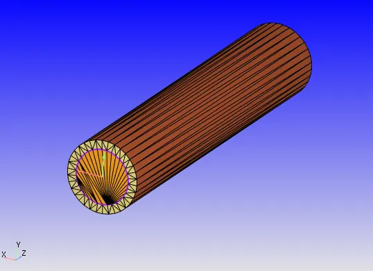
The following geometry is created in converge. The details are shown below:

Length of pipe = 0.2m

Inner Diameter = 0.015m

OuterDiameter= 0.02m

Case setup:

• Materials = Gas and solid simulation with species Air and Aluminium.
• Solver = Density based Transient solver
• Boundary = Solid outer wall-WALL, Solid side- WALL,

Inlet = INFLOW, Neumann BC for Pressure.

v = Re*mu/rho*D, Re = 7000, D = 1.225kg.m^-3, mu = 1.81e-5kg.(m.s)^-1

therefore, v = 3.45m/s

Outlet = OUTFLOW, -10000W/m^2 heat flux, NE BC for velocity.

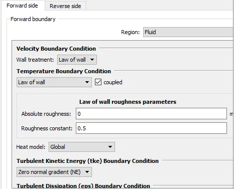
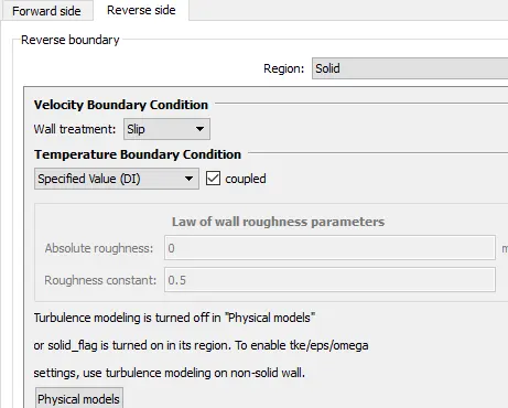
• Interface:

• Regions and Initilization: Fluid stream ID = 0 & Solid stream ID = 1
• Turbulence modelling = Rans K Epsilon
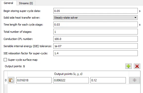
• Super-cycle modelling:

Results:

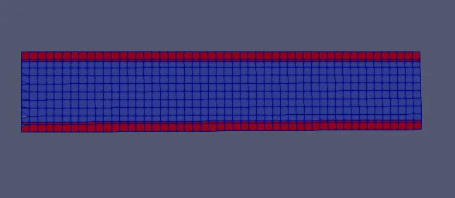
Case-1: Base grid = 0.004m

Mesh:

Temperature Contour:

Animation Link:

https://drive.google.com/file/d/1fo71ljVB9xq2COjz1Bzn6qlpOIcrwFnH/view?usp=sharing

Mean Temperature plot:

Fluid:

Solid:

Super-cycle Temperature plot:

Velocity Contour:

https://drive.google.com/file/d/1AYCLGQPlDHX_MVmJmYudaxvjDIoD4Ns1/view?usp=sharing

Pressure contour:

https://drive.google.com/file/d/1E4Juvqsn0HXXDfsMAxL7dieCL9Kkwk_g/view?usp=sharing

Y-Plus:

Case-2: Base grid = 0.01m

Temperature contour:

Animation Link:

https://drive.google.com/file/d/1MR84nlFaWA5_B5KuLBPJ7i5x1dckd6nQ/view?usp=sharing

Mean Temperature plot:

Fluid:

Solid:

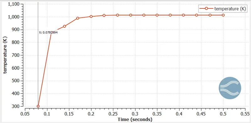
Super-cycle Temperature:

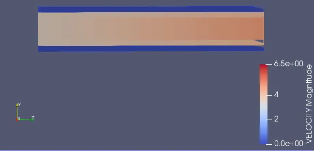
Velocity contour:

Animation link:

https://drive.google.com/file/d/1py7dbSZieiOyMEUeDOwV_u0h_b7jrdcB/view?usp=sharing

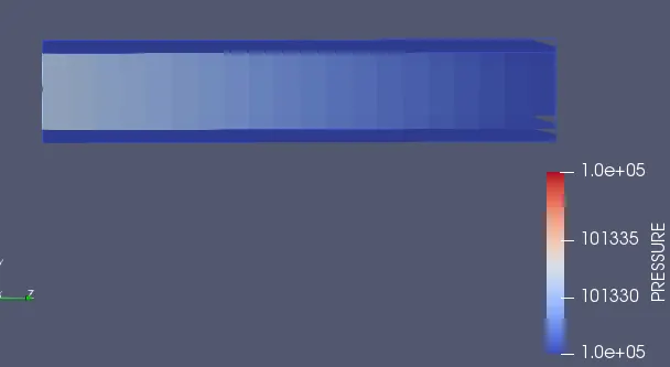
Pressure contour:

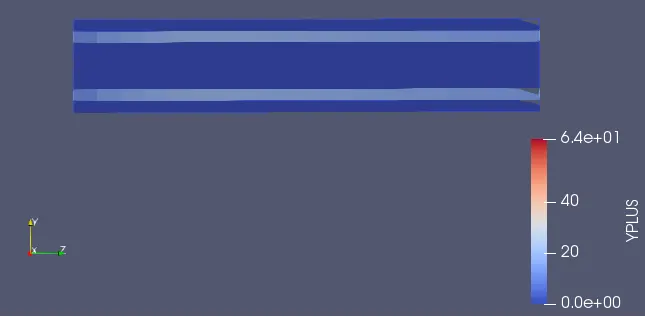
Y-Plus:

Case-3: Base grid = 0.02m

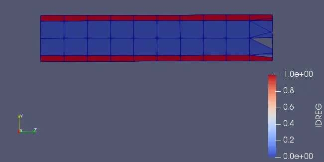
Mesh:

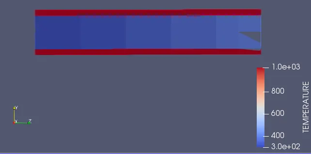
Temperature Contour:

Animation link:

https://drive.google.com/file/d/1rMGvkCg9pP7MQS0V8KtPVwJwiPbiV_5K/view?usp=sharing

Mean Temperature plot:

Fluid:

Solid:

Super-cycle Temperature:

Velocity Contour:

Pressure Contour:

Y-plus:

Discussions & Conclusion:

Three cases of different mesh sizes were used in the simulation which are 0.004, 0.01, 0.02.

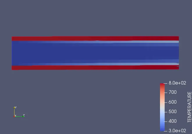
In case-1 : 0.004, the distribution of temperature is clearly seen throughout the simulation.

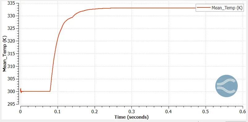
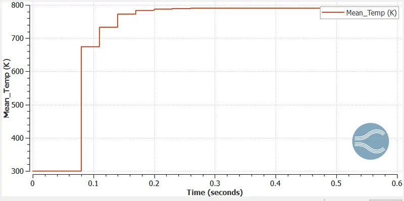
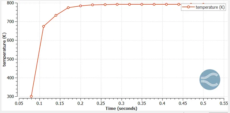
The Mean temperature of fluid is observed to be 333K and 790K for solid as well as super-cycle temperature.

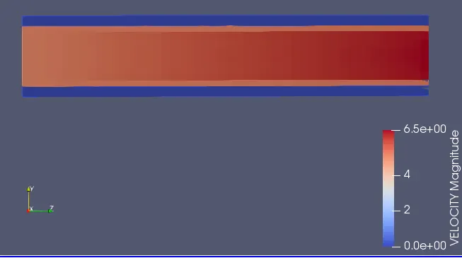
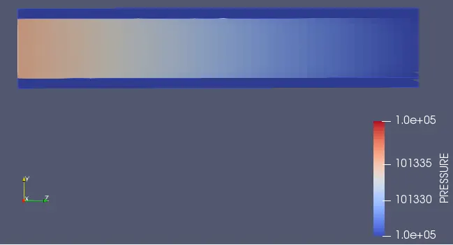
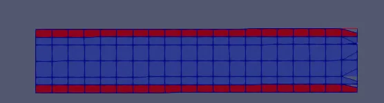
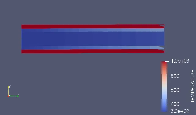
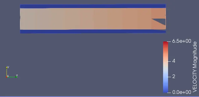
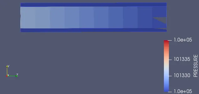
In case-2 : 0.01 & case-3 : 0.02, the distribution of temperature, pressure, velocity are not clearly good for analysis because of the very poor mesh generation which makes the flow to be disturbed.

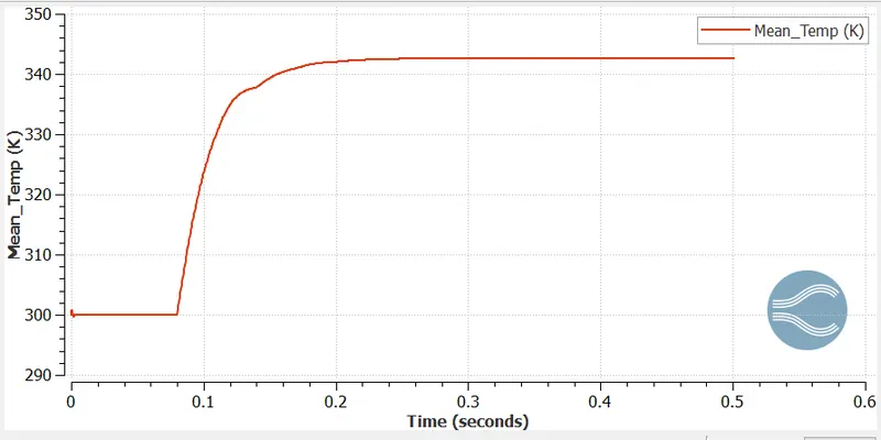
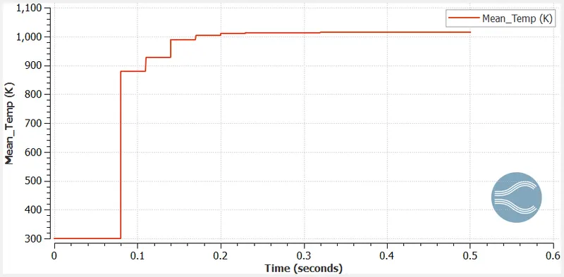
for case-2: The Mean temperature of fluid is observed to be 342K and 1013K for solid as well as super-cycle temperature.

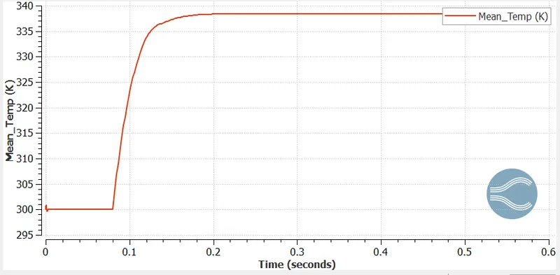
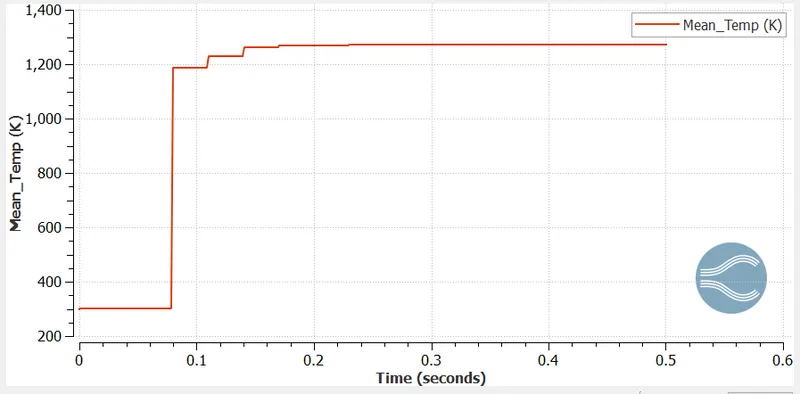
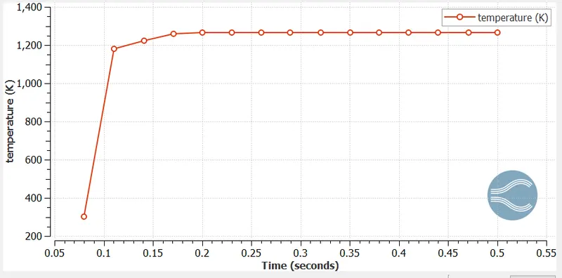
for case-3: The Mean temperature of fluid is observed to be 338K and 1266K for solid as well as super-cycle temperature.

Grid Size	Y-plus	Solid Region Temperature	Fluid Region Temperature
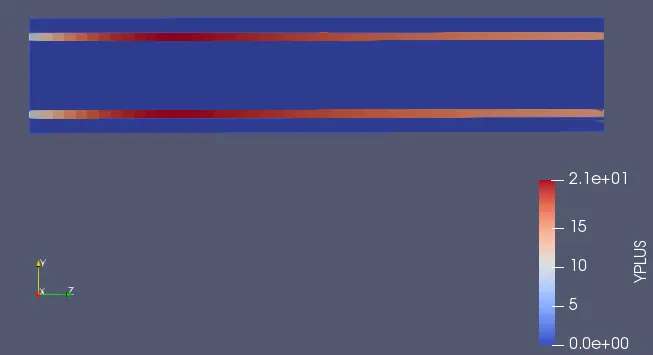
Case-1 0.004	21	790 K	333 K
Case-2 0.01	64	1013 K	342 K
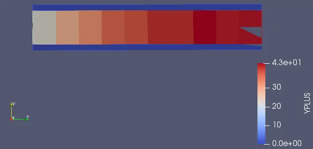
Case-3 0.02	43	1266 K	338 K

The fluid region temperature is almost not varied even though changes in mesh size. But the solid region is varied alot by changing the mesh size.

Y+ values increases as the mesh becomes coarse.