Week 6: Conjugate Heat Transfer Simulation

AIM:

To simulate a Conjugate heat transfer (CHT) analysis on a pipe.

OBJECTIVE:

To set-up a baseline configuration for flow through a pipe where inlet Reynolds number `Re = (rho*V*D)/(mu)` should be 7,000.

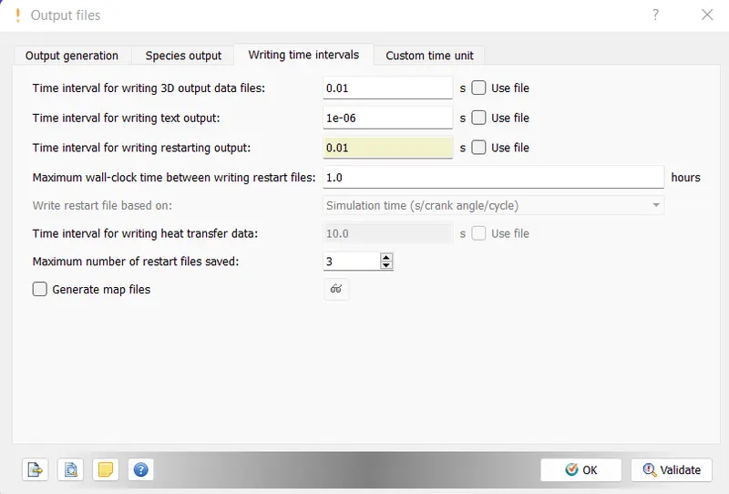
Setup model for turbulence k-epsilon with super cycling parameters for 3D outputs with super cycle stage intervals of 0.01, 0.02 and 0.02.

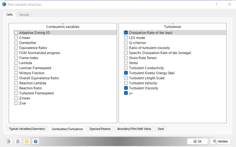
To add Y+ to post.in file and do the grid independence test for any 3 base grid sizes.

DESCRIPTION:

CONJUGATE HEAT TRANSFER:

Cojugate heat transfer is used to describe the processes which involve variations of temperature within the solids and fluids due to thermal interaction between the solids and fluids.

The CHT analysis is generally used in places whwre there is heat transfer taking place for example when a fluid flows through a pipe and the heat of the fluid is transferred to the pipe by convection. CHT analysis is very much useful in analyzing the areas where there are two bodies in which heat transfer takes place. when this analysis is used it is easy to calculate the heat transfer coefficient, temperature and velocity of the fluid flowing through a certain body.

This type of heat transfer corresponds to the combination of heat transfer in solids and heat transfer in fluids. Heat transfer in solids is called conduction and heat transfer in fluids is called convection.

Conduction occurs due to the direct molecular collision, the faster kinetic energy collides with the low-speed kinetic energy and heat transfer occurs.

The convection process is not happening alone. It is combines with the conduction or radiation. It occurs mostly in the cooling process like heat sink, battery cooling, airflow over the solid object for cooling.

SUPER-CYCLING:

Super-cycling is a method used in converge studio for CHt problems with multi-phase regions i.e for solids and liquids. The solvers for different fluids cannot run at the same speed for solving the fluid it is much faster compared to solids. If this is done the solution does not reach convergence. So, super cycling can be used to resolve this issue. This helps solver of fluid domain is paused until the solver for solid converges.

THEORY FOR Y+:

Wall functions are useful in assigning the solver how to approach the solution near the wall. This helps in predicting the turbulence models for the coarse grid. No-slip condition is used if the flow is completely laminar that does not depends on grid size. For turbulent flows, the laminar region is very small to get accurate results so we need a very small grid size near the boundaries. This is where the Y+ values help.

Y+ is a non-dimensional term that can be used to understand the grid is finer or coarse. This can be used to determine if wall functions are used or not. In viscous sub-layer Y+ is less than 10 and in turbulent region Y+ is greater than 30.

STEPS FOR SIMULATION OF CHT ANALYSIS:

Here we set up a simulation for a case such that a solid pipe is heated by external flux.

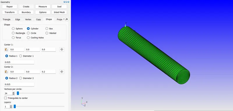
Creating a geometry with Radius of 0.015m and length in z-direction as 0.2m using Create>Shape>cylinder

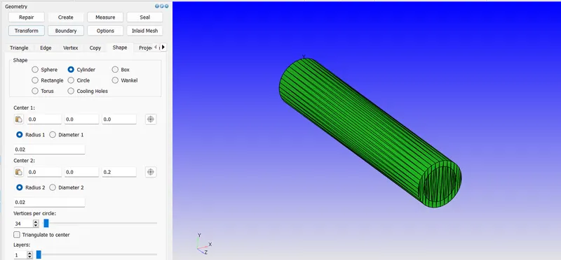
adding the thickness of 0.02m as we need a solid

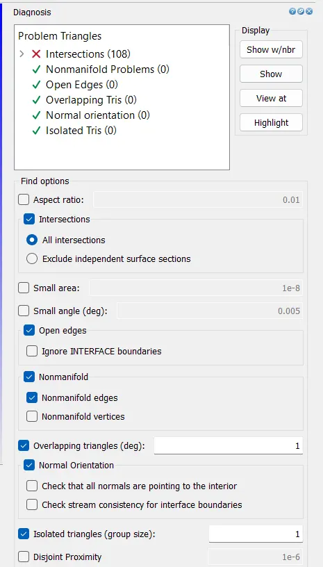
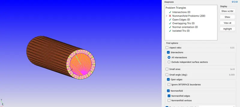
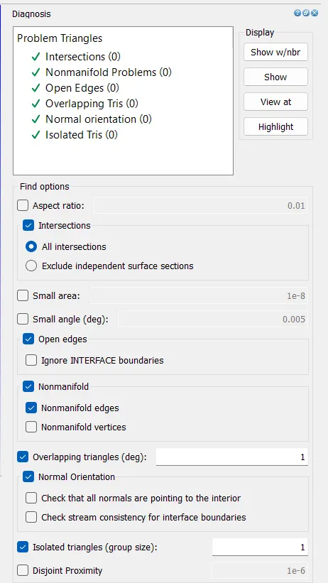
Running the diagnosis we get intersection errors

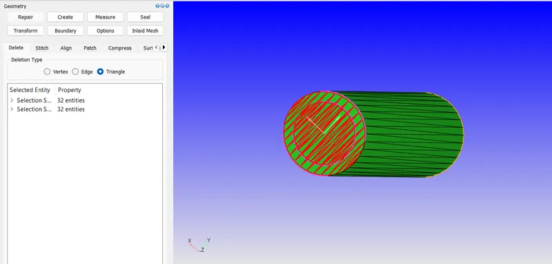
So to delete the intersecting triangles using Repair>delete>triangle selection with angles

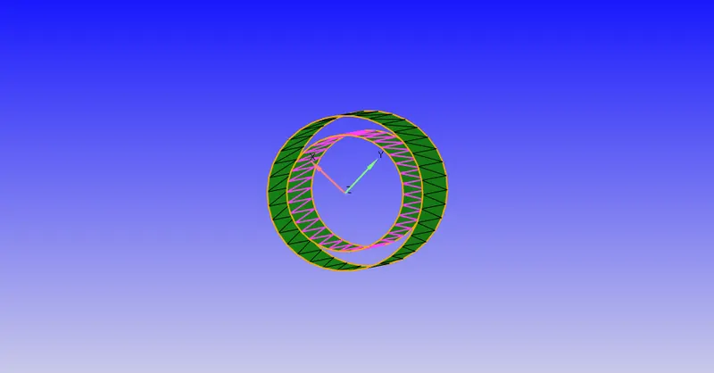
Now we need to create boundaries which represent the thickness of the solid and the inlet

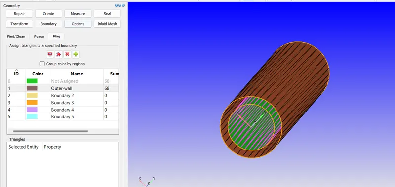
For outer wall to which heat flux will be applied

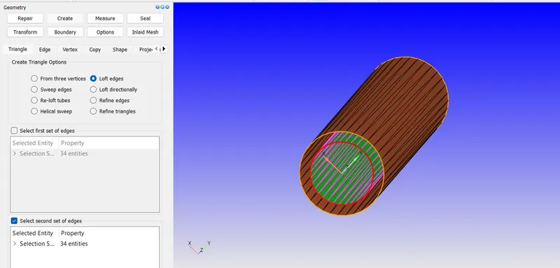
Now creating the thickness using Create>Triangles>Loft edges and select the edges

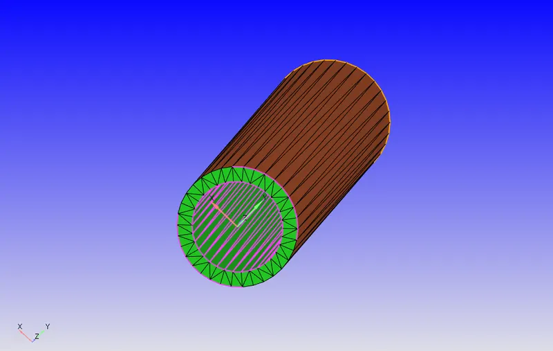
Adding to boundary

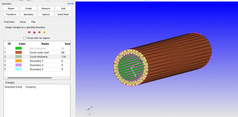
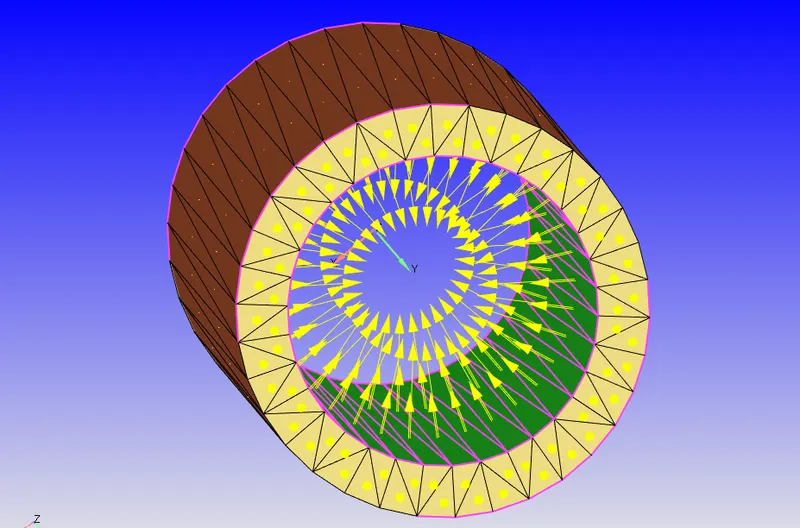
Now looking for normals we see they are pointing inside

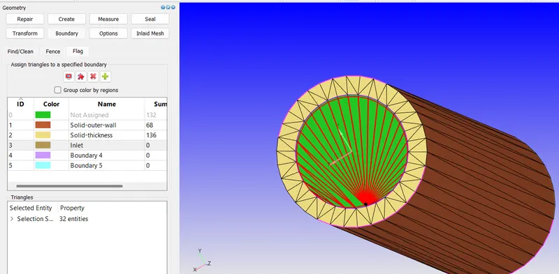
Now creating the inlet & outlet using Repair>patch>list of edges using Arc selection

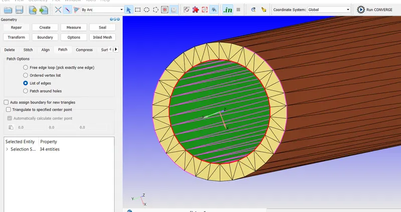
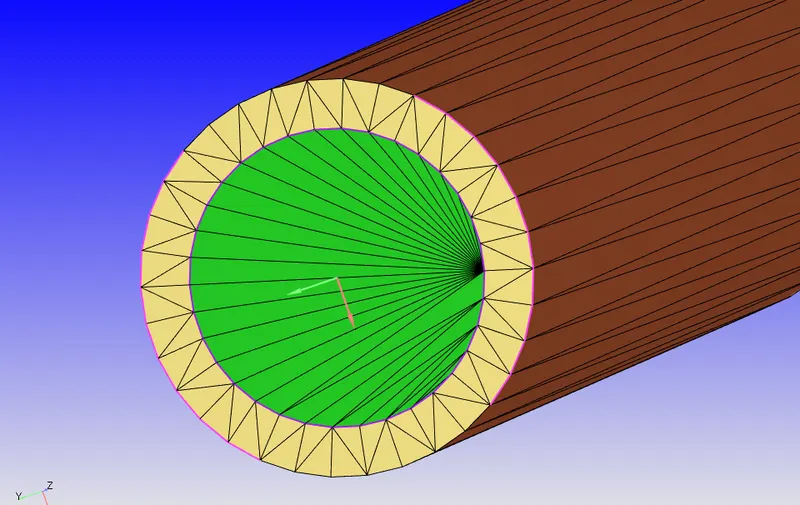
For Inlet

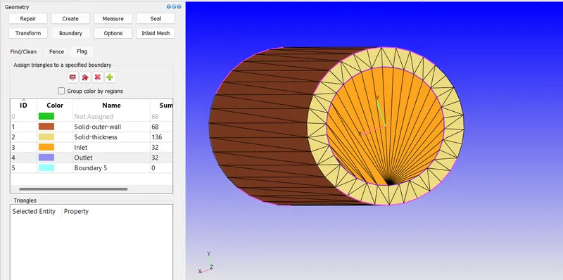
For Outlet

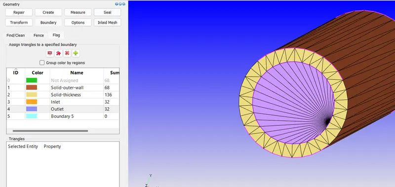
For interface boundary

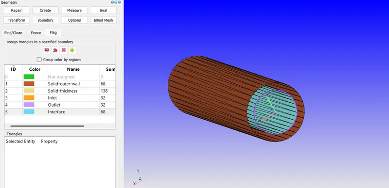
Now checking the diagnosis we see manifold erros and we get them for CHT analysis are one edge is being shared between the solid and fluid and the inlet and outlet

Now setting up the case

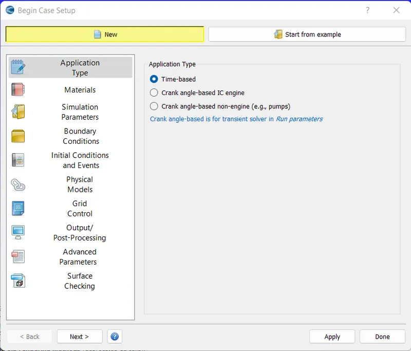
General type-time based case set-up

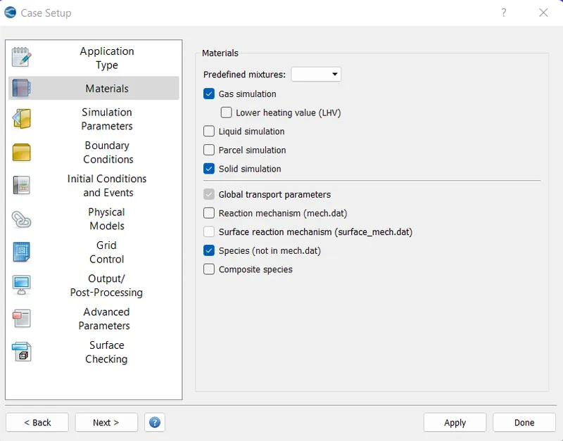
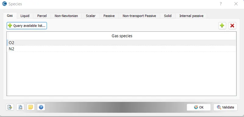
For materials, we have fluid as Gas simulation and also solid simulation and Air with species enabled

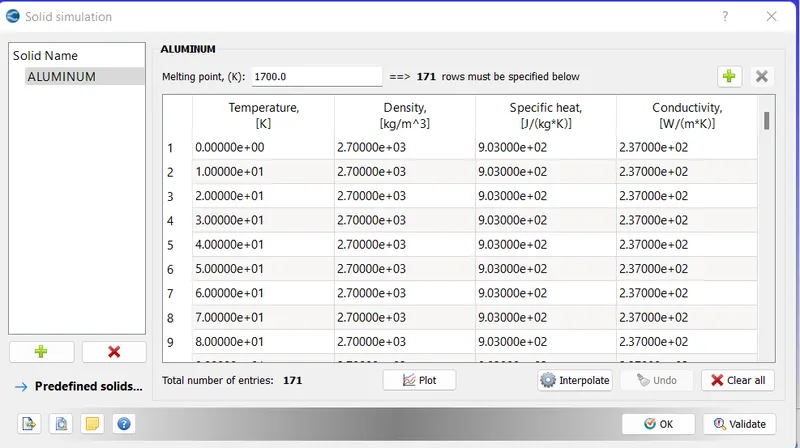
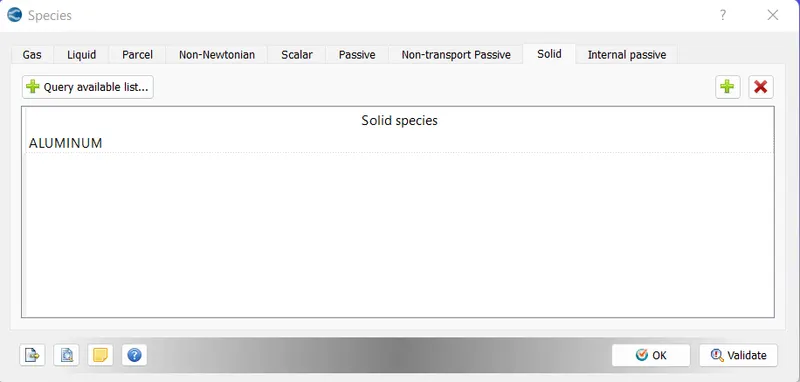
Solid simulation we go for Aluminium

For species

For solid species, we select Query available as Aluminium

And for Gas, O2 and N2 i.e Air

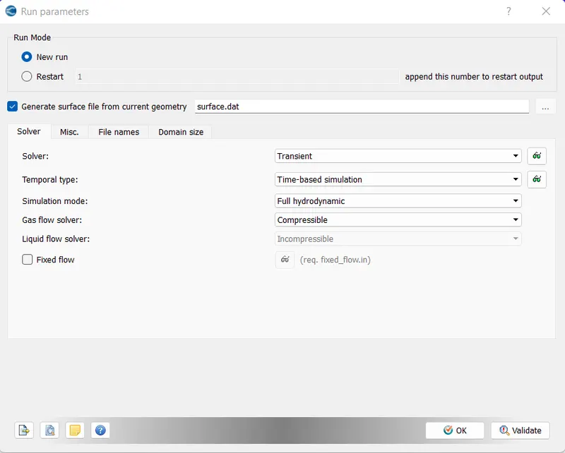
Run parameters, with Transient and full hydrodynamic with compressible

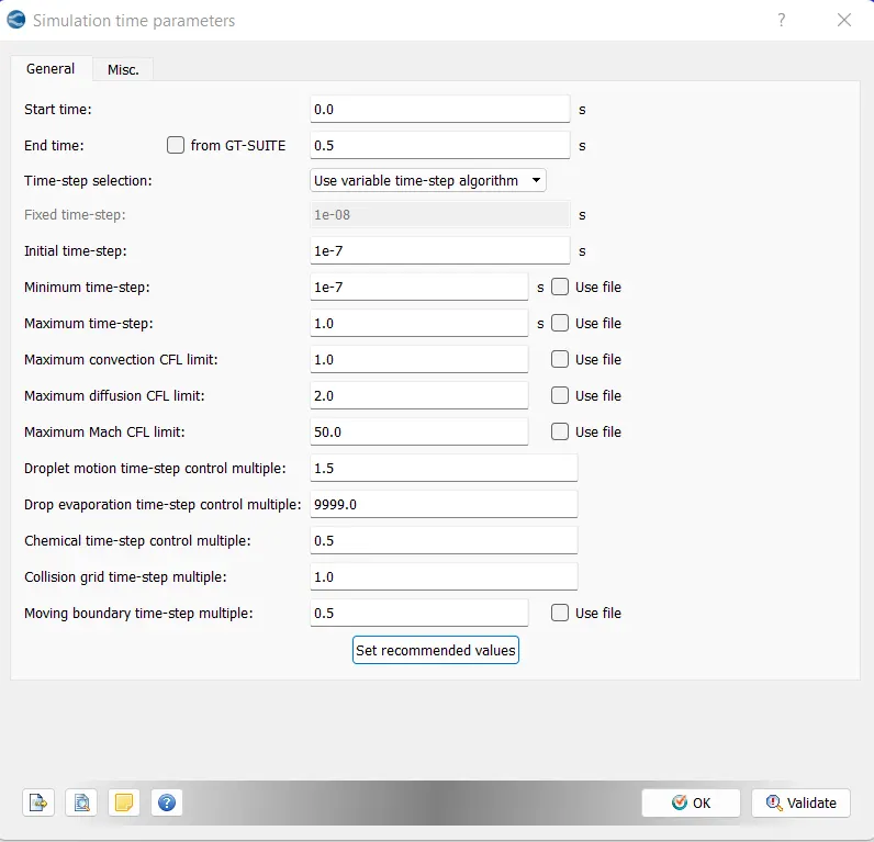
Simulation time parameters

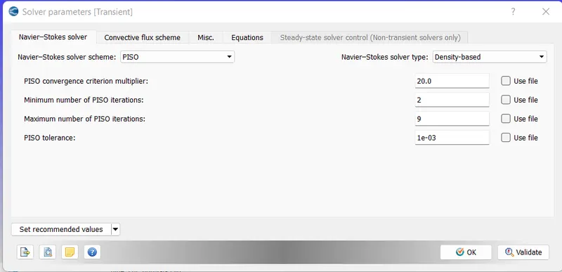
Solver parameters as default

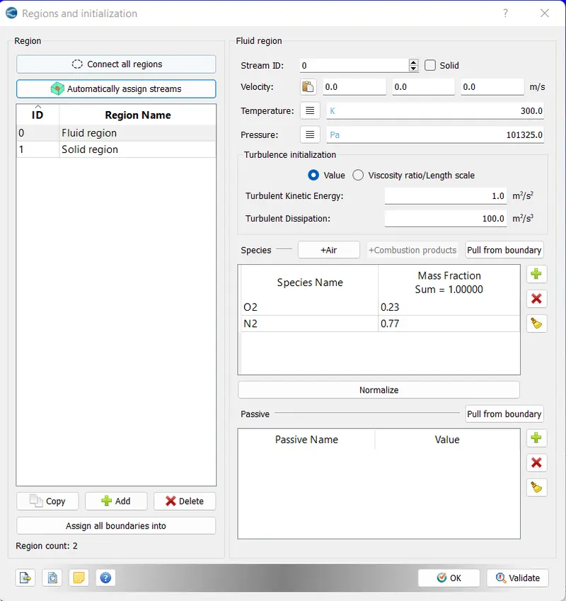
For Regions and Initialization

For fluid region, with Air

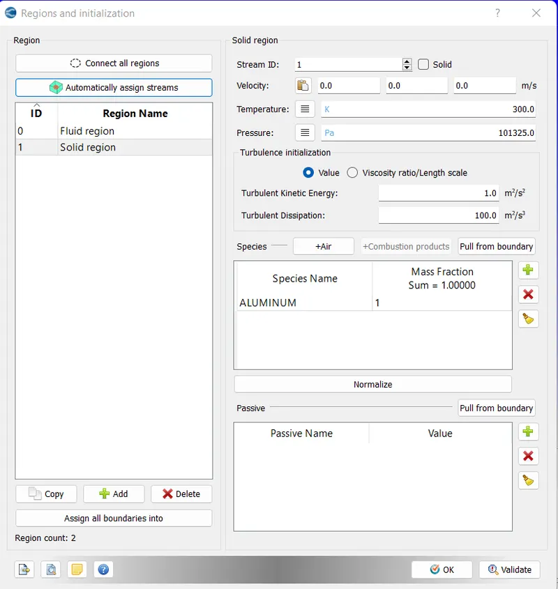
For Solid region with stream ID 1 and solid checked with Aluminium

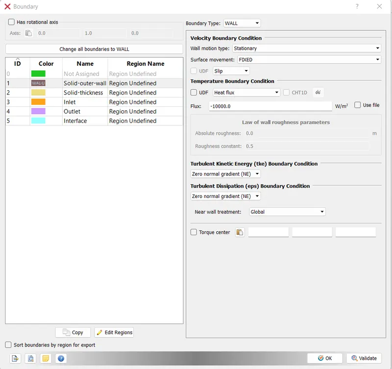
Boundary conditions

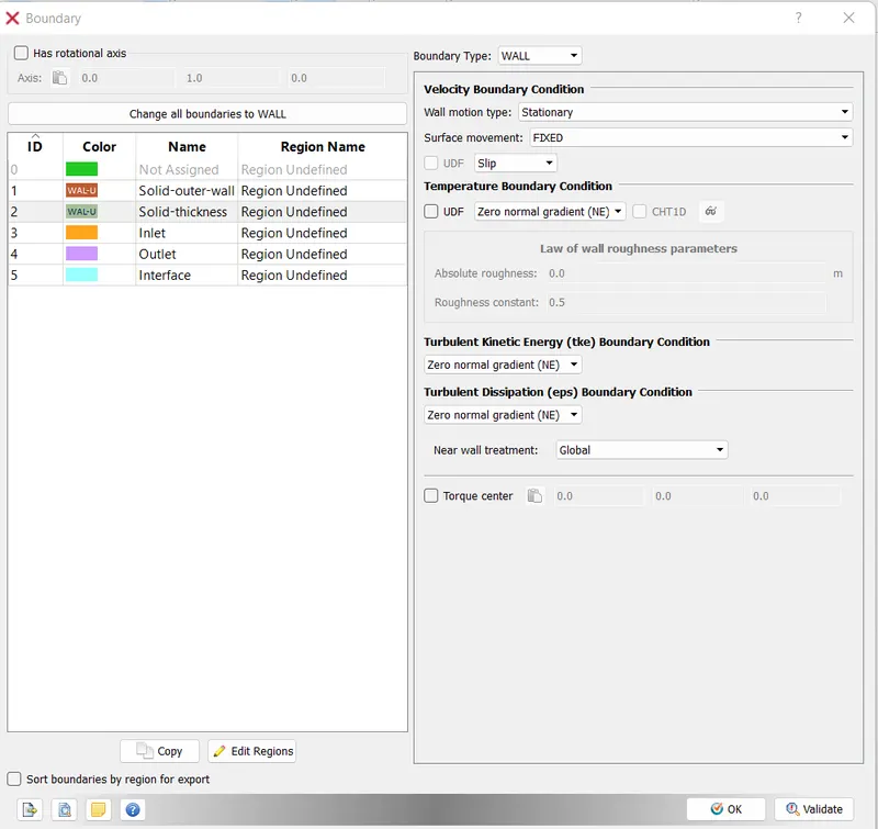
For Outer solid surface, we use stationary wall fixed with slip and not Law of wall as its used for fluids and heat flux flowing inwards (external heat) with -10000 W/m2

For solid thickness, wall with velocity slip and temperature adiabatic i.e zero normal gradient

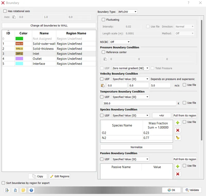
For inlet,Inflow with pressure Neumann BC and velocity 5m/s in +ve z-direction with Air

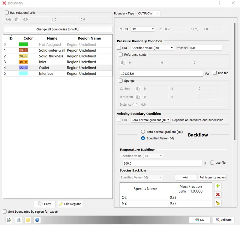
For Outlet, with outflow and static pressure of 101325Pa and Backflow as Air

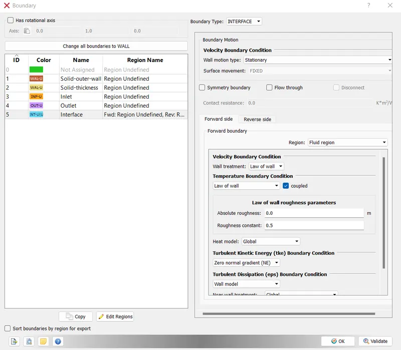
For interface, as Normals as pointing inwards which is a forward boundary i.e fluid and if pointing outwards it would have been solid forward

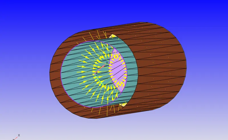
For forward side, with fluid region normal pointing and Law of wall for fluid velocity and temperature

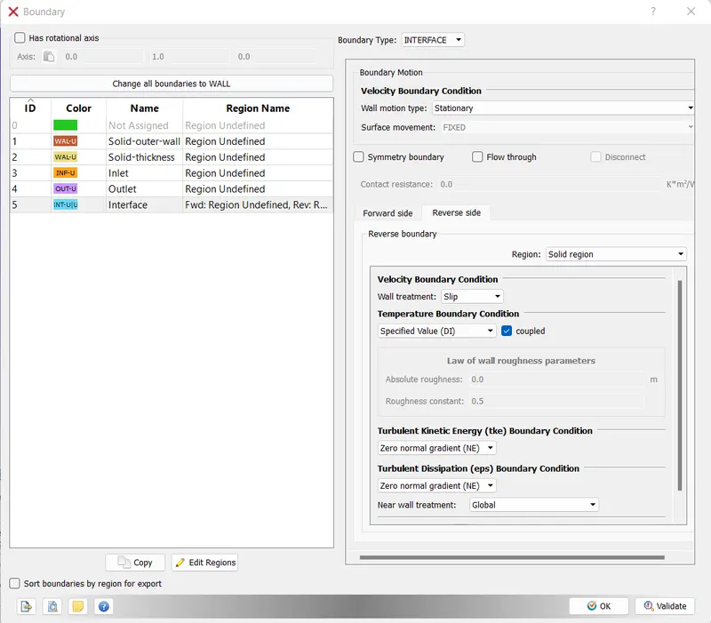
For Reverse side,Region is solid region and law of wall BC for velocity and for temperature specified value

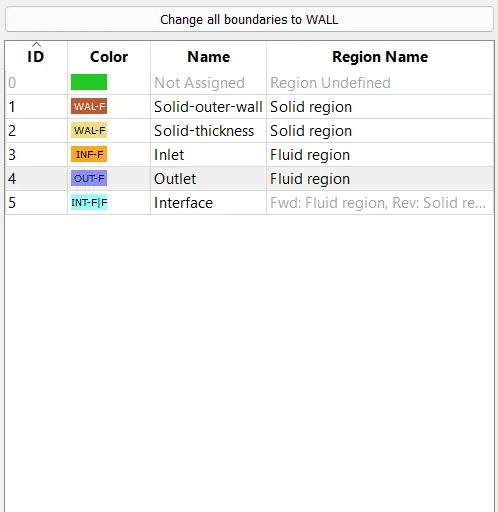
Assigning the regions to BCs

Now for setting up the model, we go for super-cycling for CHT analysis

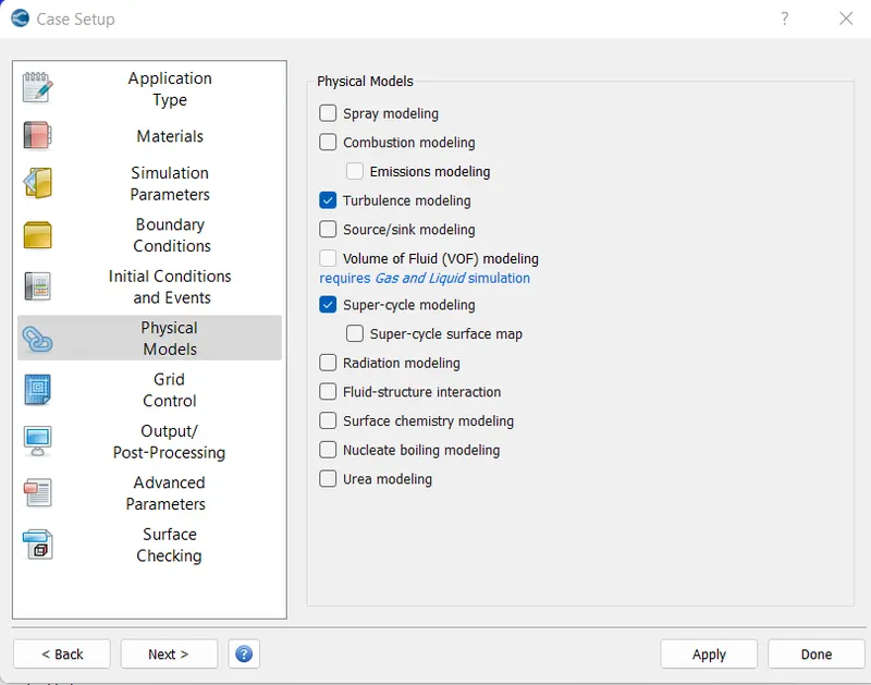
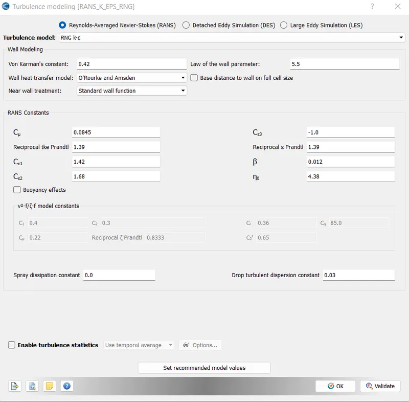
Turbulence model with default RNG k-epsilon

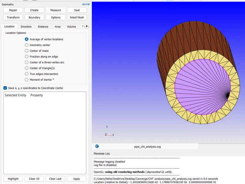
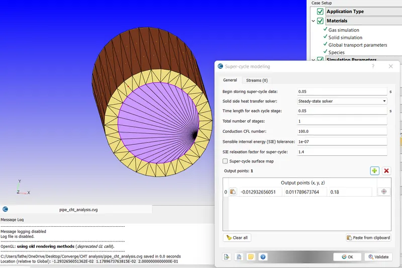
For super-cycling, measuring by using Location>Average of vertec locations and selecting two vertices on outlet side of the thickness of surface

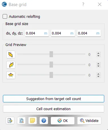
For Base Grid, for case-1 4mm and for case-2 3mm and for Case-3 with 2mm

For post-processing adding Y+

For Outpt files

Now running the diagnosis we see no errors as Converge studio has recognised the case set-up as CHT analysis based on the case set-up

Then running the case set-up after exporting the input files to the folder using Cygwin.

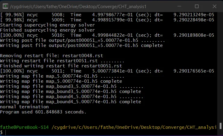
By using the application mpiexec.exe & converge.exe by command line 'mpiexec.exe -n 2 converge.exe restricted' we run the simulation till results are converged.

Then using converge and paraview post processing results are observed and studied.

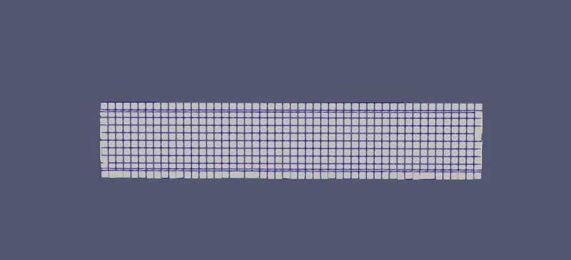
CASE-1: WITH MESH 4MM

The Mesh is as follows

The Velocity contour is

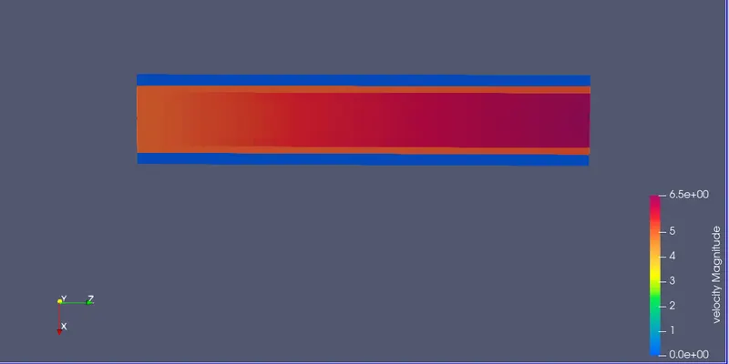
The Velocity Animation is

The Pressure contour is

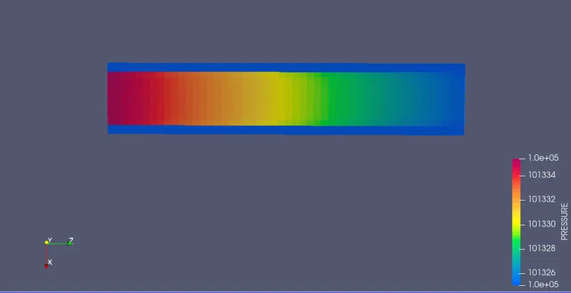
The Pressure Animation is

The Temperature contour is

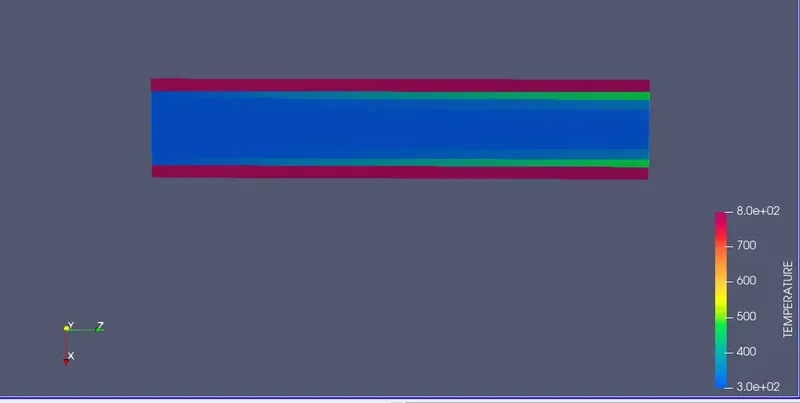
The Y+ contour is

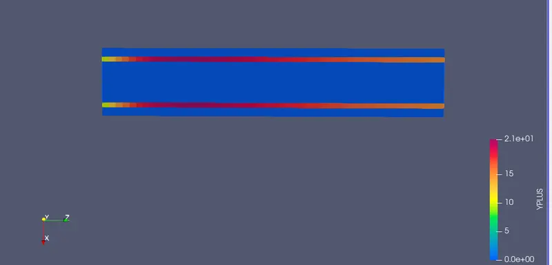
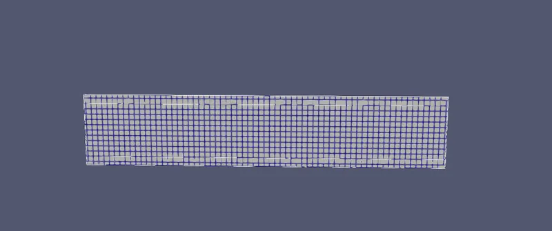
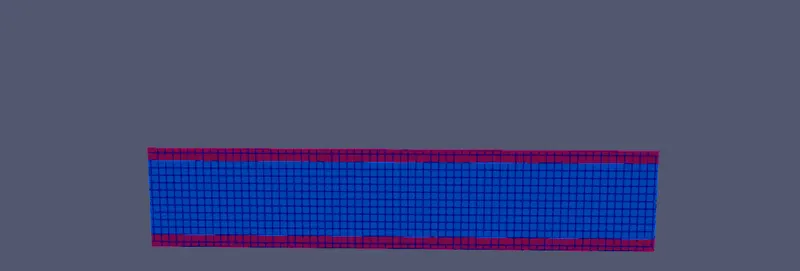
CASE-2: WITH MESH 3MM

The Mesh is as follows

The Velocity contour is

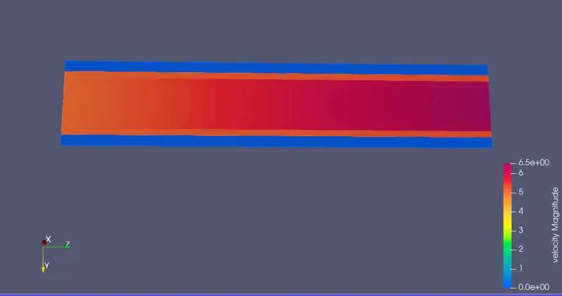
The Velocity Animation is

The Pressure contour is

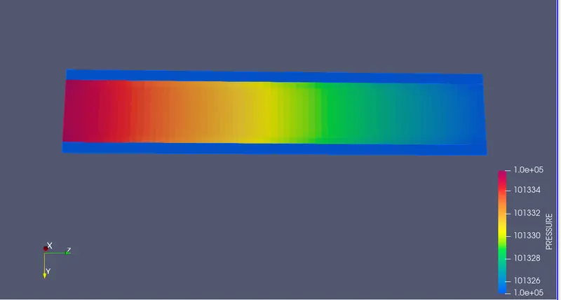
The Pressure Animation is

The Temperature contour is

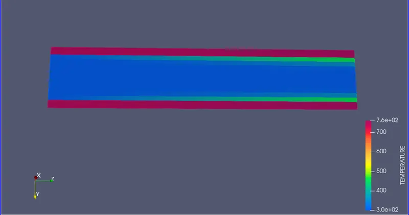
The Y+ contour is

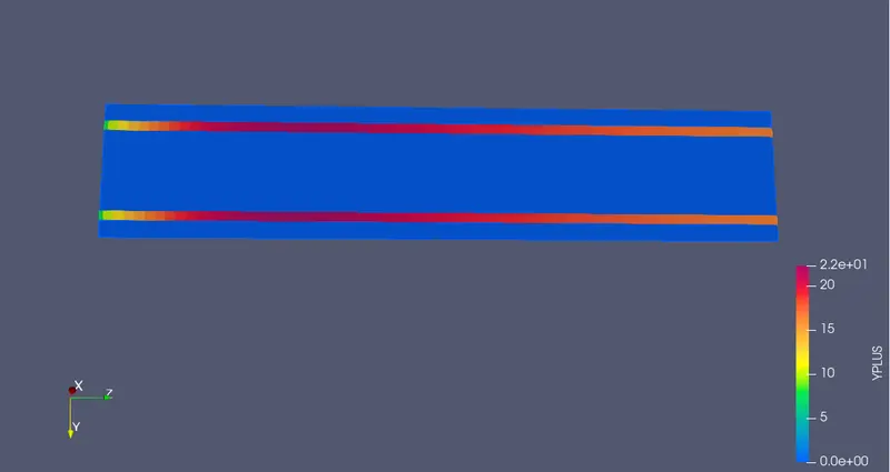
CASE-3: WITH MESH 2MM

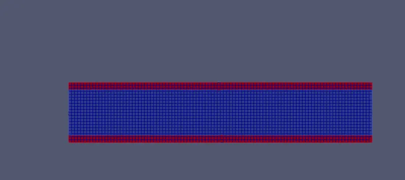
The Mesh is as follows

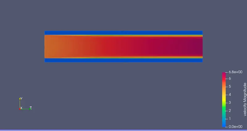
The Velocity contour is

The Velocity Animation is

The Pressure contour is

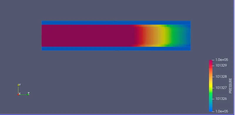
The Pressure Animation is

The Temperature contour is

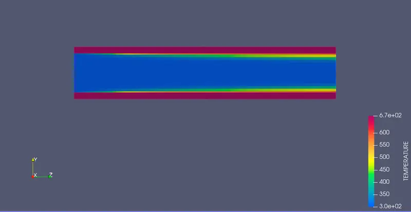
The Y+ contour is

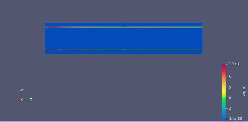
BASED ON SUPER-CYCLING:

For Case-1

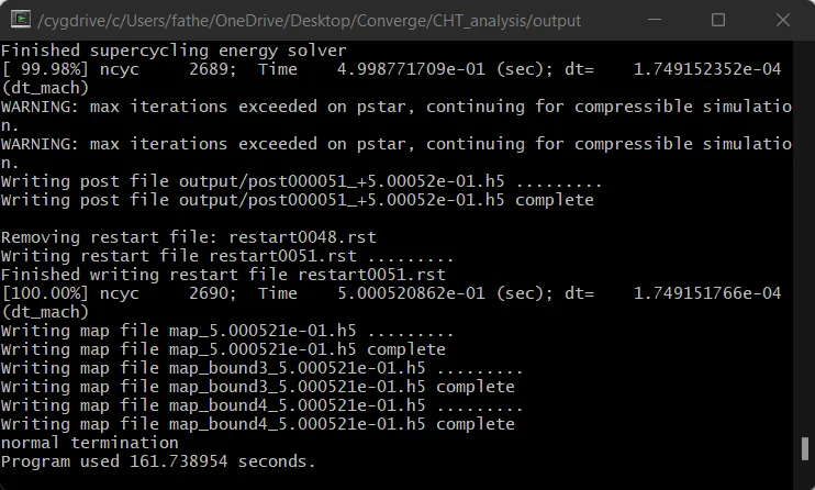
For Case-2

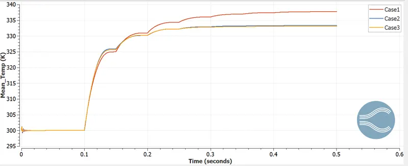
FLUID REGION MEAN TEMPERATURE:

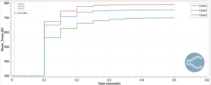
SOLID REGION MEAN TEMPERATURE:

CONCLUSION:

Refinement of grid size results in clearer plots and contours but consumes higher computational time.

Decreasing the super-cycling time interval results in reduction of computational time and if just changed the mesh grid size for same Super-cycling time interval we see increase in computational time.

Irrespective of grid sizes, fluid values converge to a temperature of 332-337K