Week 6 - CHT Analysis on a Graphics card

Aim:-

To Perform a steady-state conjugate heat transfer analysis on a graphics card model. You can use appropriate materials of your choice for the simulation. Could you make sure to define the correct solid and fluid zones properly?

Simulate the best possible mesh with a combination of coarse and refined mesh in different regions. Explain the reason for choosing the particular mesh settings.

Objective:

• To import the graphics card model into spaceclaim and perform share topology.
• To generate the mesh for the graphics card model by selecting different mesh element sizes for various cases and performing the grid independence test.
• To set up the simulation by assigning the required materials for different cell zone regions of the model and providing the heat generation rate from the processor as the heat source.
• And to provide the required boundary condition for all the regions of the model and vary its inlet velocity for different cases of simulation.
• Finally post-process the result.

Introduction:

We will simulate the flow over a given graphics card model and perform the CHT analysis on the graphics card. In real-world applications, the processor in the graphics card generates heat which is reduced by the flow of air over the processor by use of the cooling fan present in some computers. Also, it increases the heat transfer rate of the processor with the surrounding air flowing over it. the fins are placed above the processor. The fins are an extended surface that increases the heat transfer rate utilizing convection. so, the heat is dissipated to the air flowing around it. It also performs the CHT analysis for different cases by varies of air 1m/s and 3m/s and 5m/s and we need to compare the results.

CHT Analysis:-

Conjugate heat transfer is the analysis of heat transfer involved in both fluid and solid simultaneously. For solving the CHT problem, we use both conduction and convection equations for the relevant phase of the material.

CHT corresponds with the combination of heat transfer in solid and heat transfer in fluid. In solid, conduction often dominates whereas in fluid, convection often dominates.

Power density:-

Power density is the amount of heat generation rate per unit volume.

So, the power density of the processor = CPU Heat generation rate of the processor / Total volume of the processor.

Case setup:-

• Here we simulate four different cases. The first two cases are for performing the mesh independency study with baseline mesh and refined mesh for an inlet velocity of 3m/s. Then choose the refined mesh for performing the simulation by varying the inlet velocity of 1m/s and 5m/s.
• We used the K-Omega SST turbulence model selected for this simulation Since the CHT analysis is focused on the graphics card region for which the K-Omega SST will give more accurate results for the near wall conditions.
• We take the processor as the heat source. Assume the heat generation rate by the processor as 70 Watts. The volume of the processor can be determined by measuring its dimension in SpaceClaim,

Hence the power density of the processor can be written as,

power density of the processor = 3 / 0.008 * 0.008 * 0.001

the power density of the processor = 46875000 W/m^3

So, this value should be given under the processor's cell zone condition, which is taken as the heat source for this simulation.

materials and their properties for different components of the graphics card:-

For fins, the primary material chosen is aluminum.

Density = 2719 kg/m^3

Cp (Specific heat) = 871 J/(Kg k)

Thermal conductivity = 202.4 W/(m k)

For fins, the secondary material chosen is copper.

Density = 8978 kg/m^3

Cp (Specific heat) = 381 J/(Kg k)

Thermal conductivity = 387.6 W/(m k)

For the processor, the material chosen is silicon.

Density = 2330 kg/m^3

Cp (Specific heat) = 703 J/(Kg k)

Thermal conductivity = 153 W/(m k)

For PCB (Printed circuit board), the material chosen is FR4.

Density = 1850 kg/m^3

Cp (Specific heat) = 4184 J/(Kg k)

Thermal conductivity = 0.25 W/(m k)

Procedure:

Case:-1 (Baseline mesh, v=3 m/s)

Geomentry:

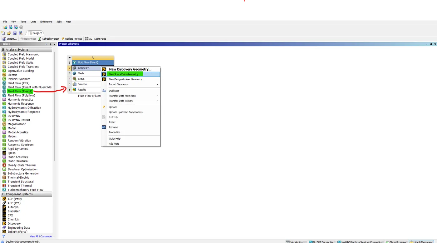
• Open the Ansys Workbench, drag the fluent flow model, open the geomentry in SpaceClaim, and drag & drop the graphics card model in geomentry.

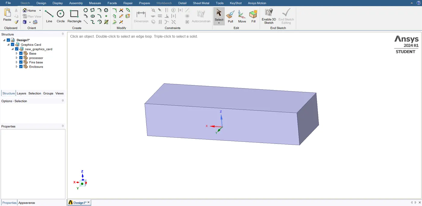
• Now you can see an encloser already present so we don't need to build an encloser separately.

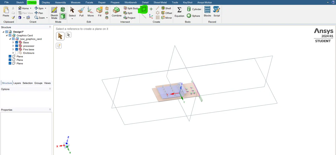
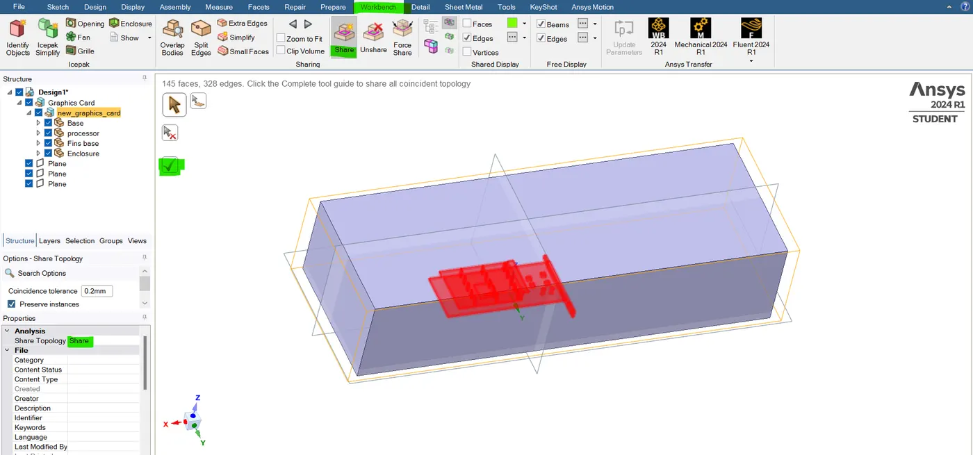
• Now we need to enable the "share topology" for this model. Once we enable a shared topology, it will indicate in pink color at the edge and also it will share the data between the enclosure and other components.

Meshing:-

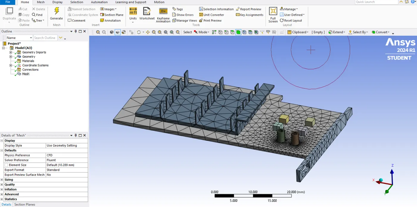
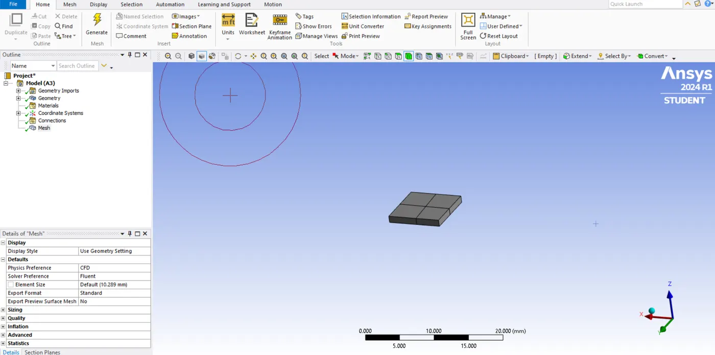
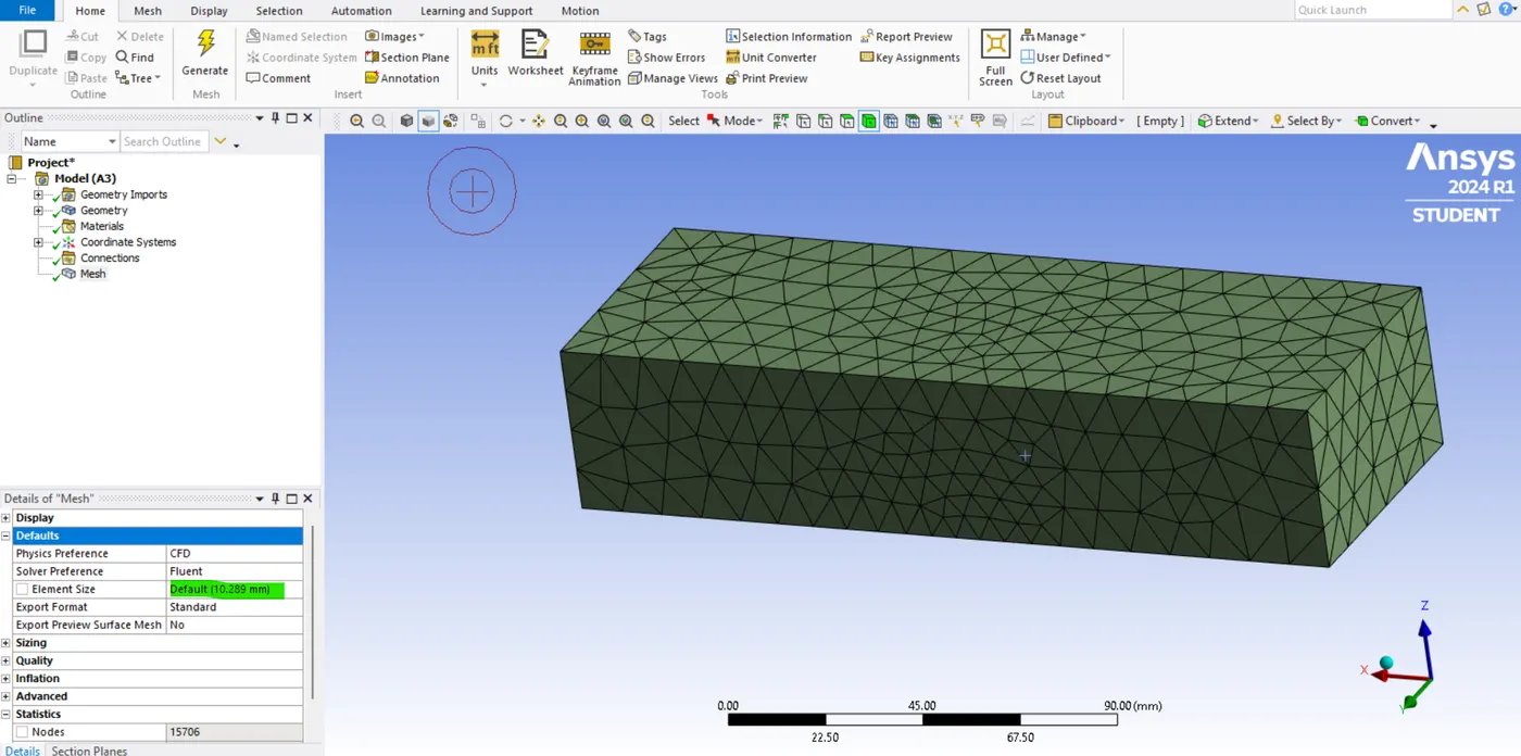
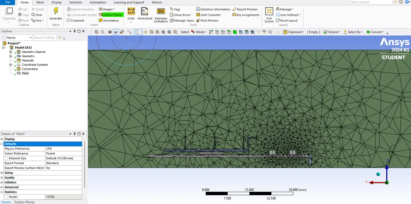
• Now we will move towards the meshing module. Here we are just performing the baseline mesh. so, we don't want to change any mesh size here. we can leave it as it is.
• so just click on generate the mesh. Let's see what it looks like.

Graphics card:

Processor:

• Encloser:

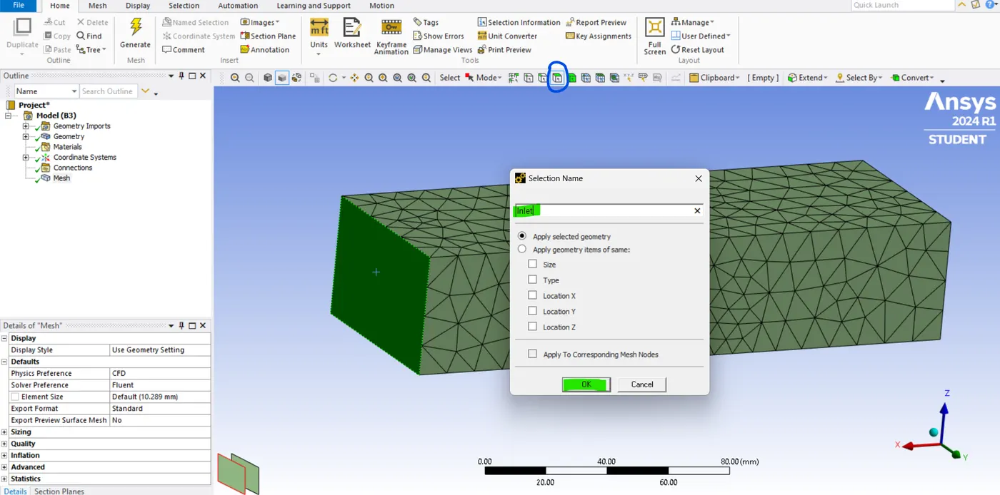
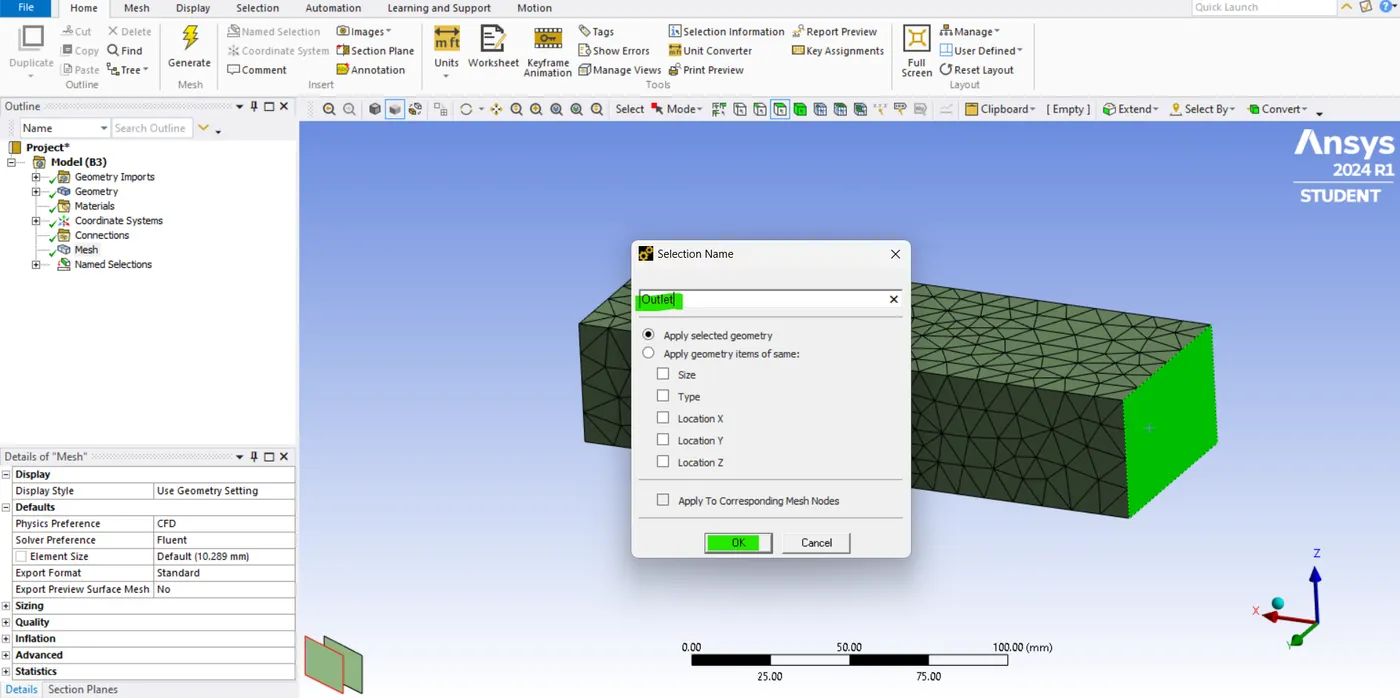
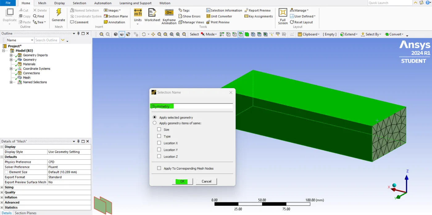
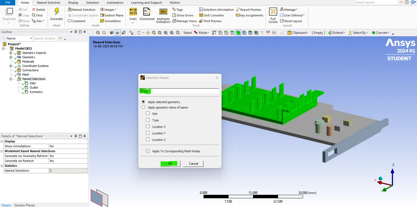
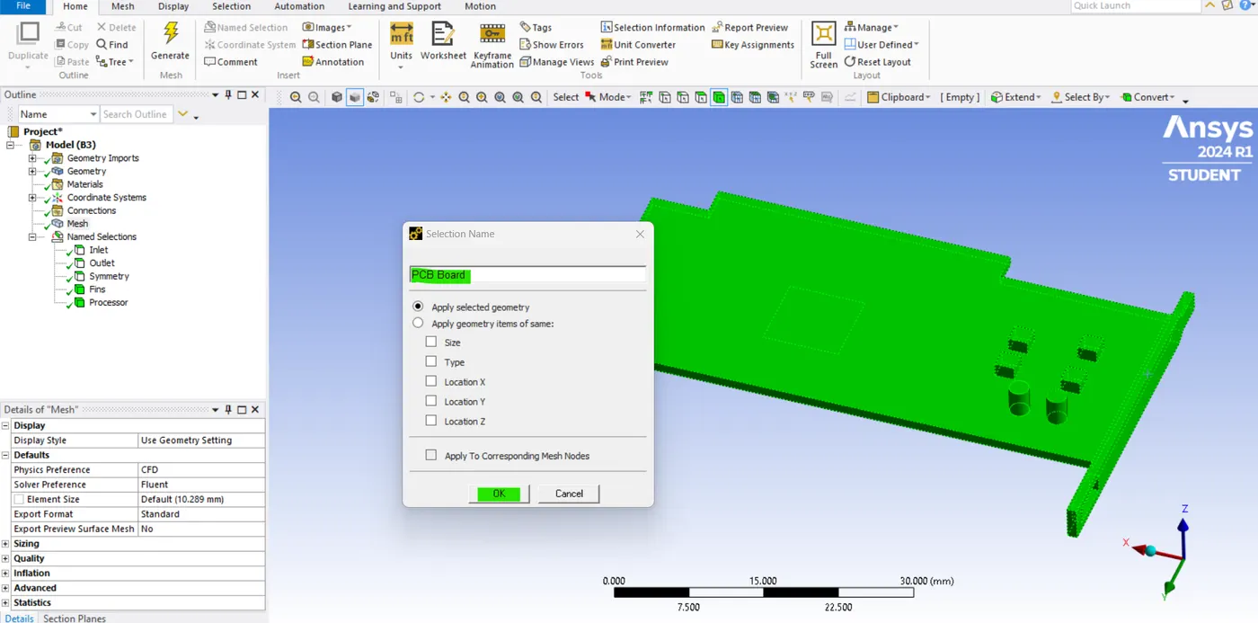
• Now we need to give name selection to the whole body.
• Inlet:

• Outlet:

• Symmetry:

• Fins:

• Processor:

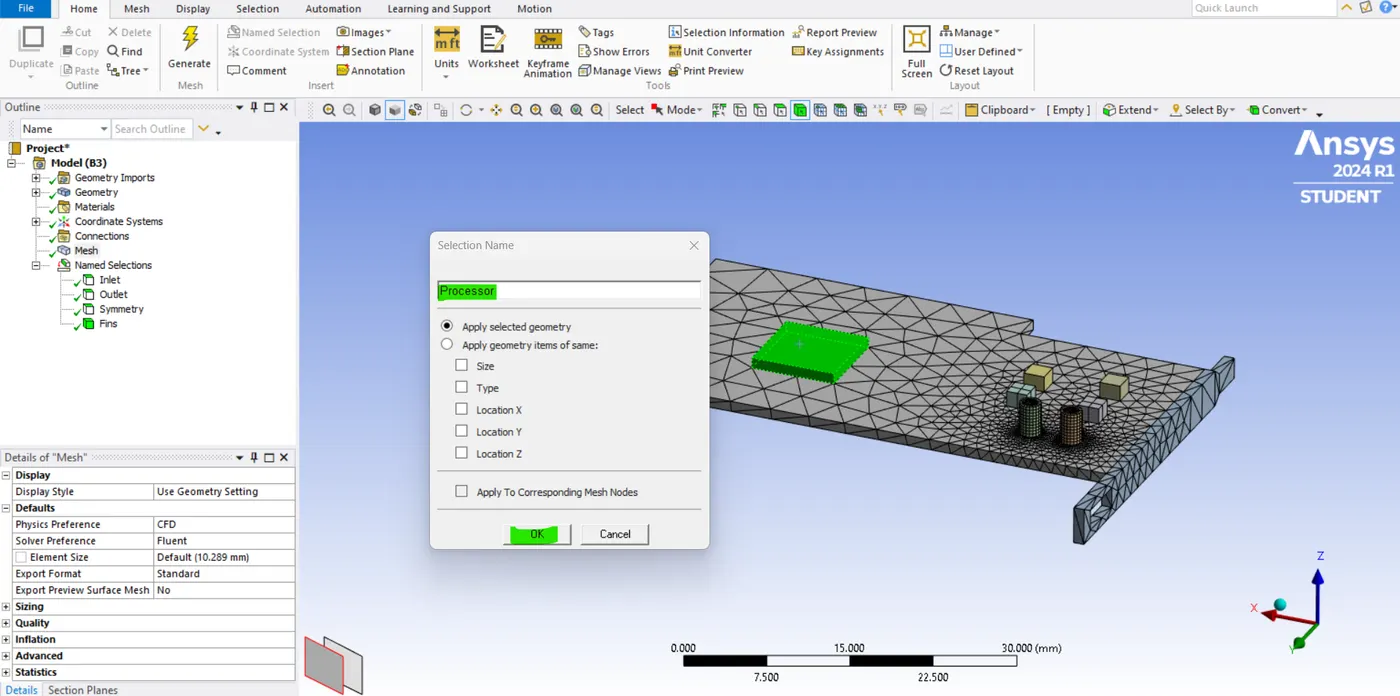
• Graphics card:

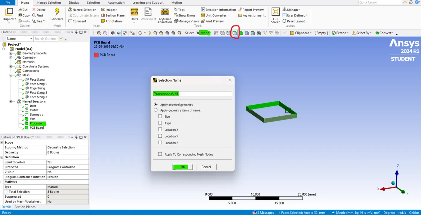
• Processor-wall:

• Mesh Metrics:

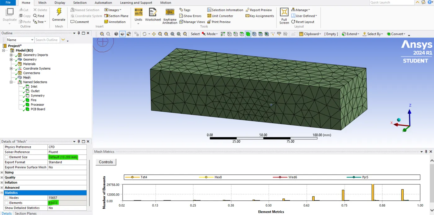
• So, the total number of mesh elements is 83472.

Setup & Solving approach:-

• Now we will move towards the set-up window.

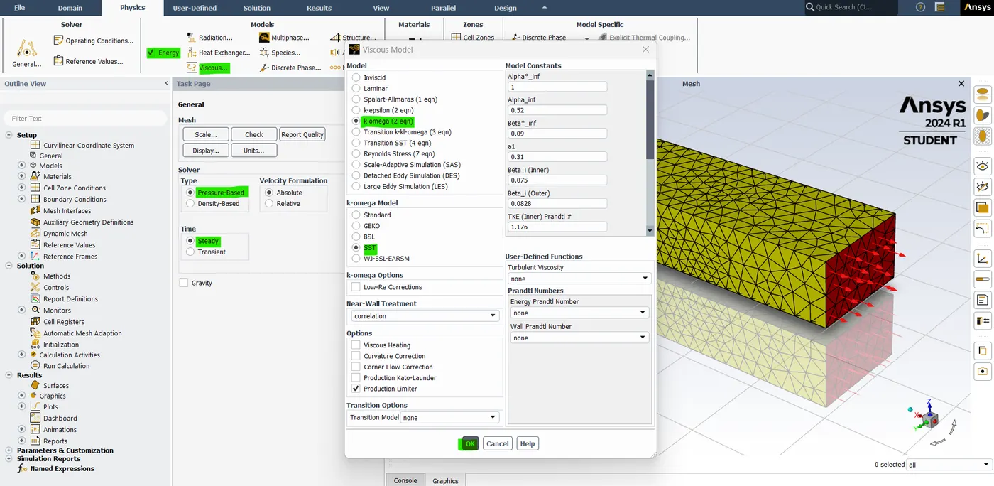
• Enable the energy by checking the tick mark and then assign the pressure-based solver and steady-state model.
• Here we use K-Omega SST Terbulance model.

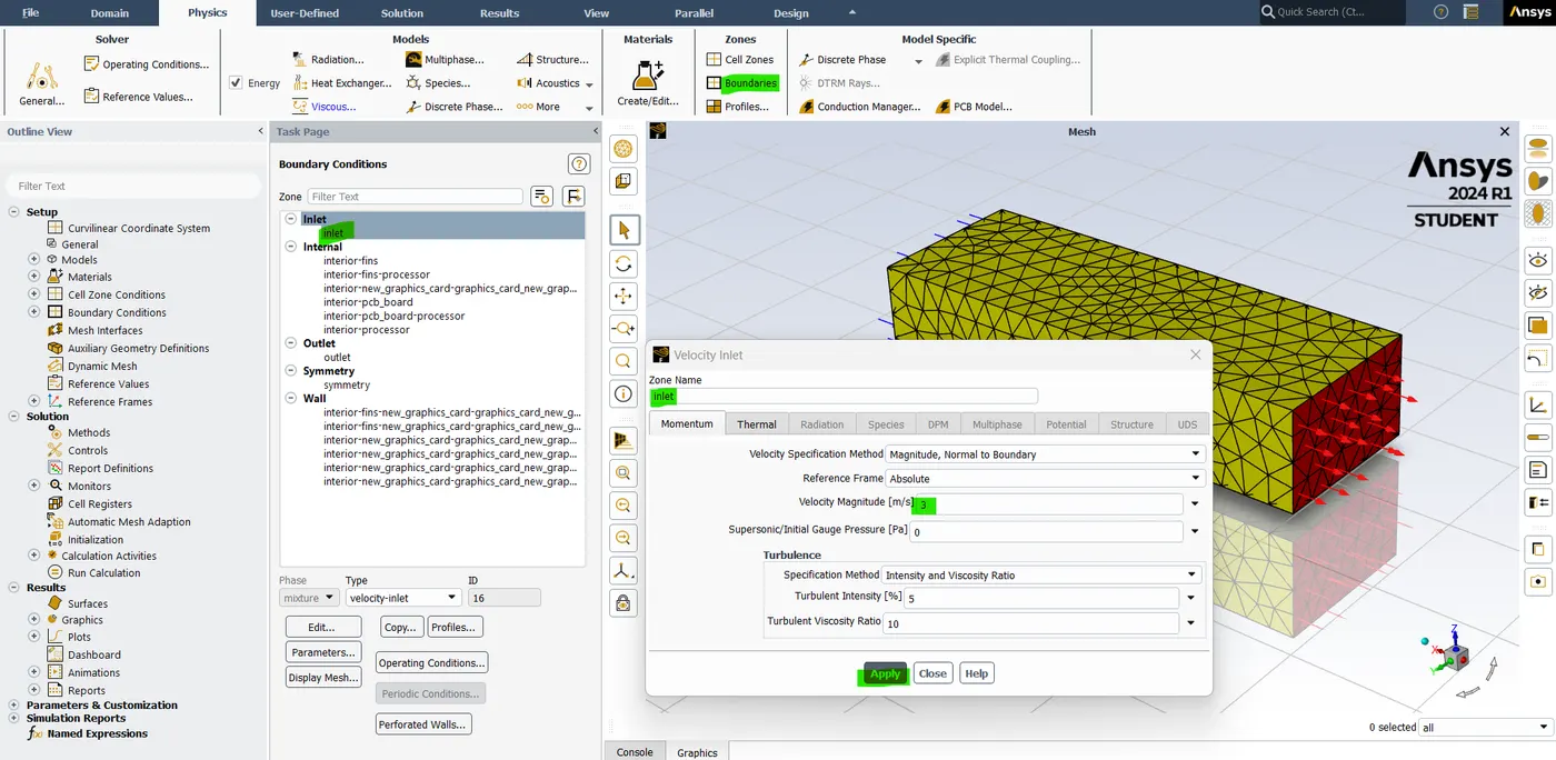
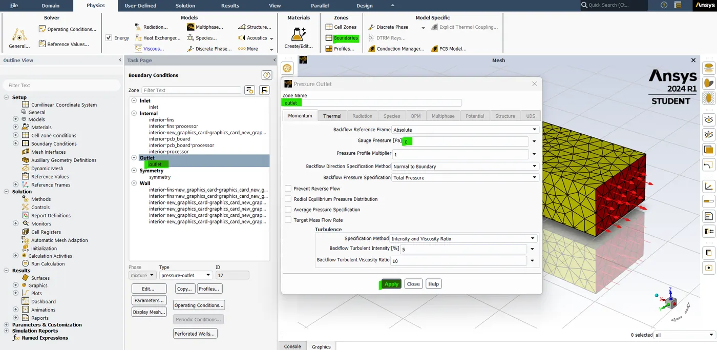
• Here assign the boundary conditions for Inlet is 3m/s and the outlet is 0m/s. And then hit apply.
• Now we need to add new materials for different components in the material list by copying one material's properties and naming them as other materials.

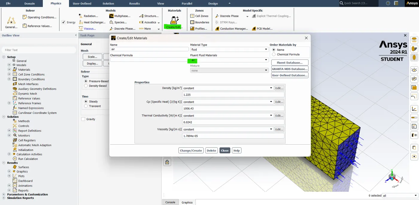
• Now go to create material and then select "air" material in fluid material type. After that hit apply.

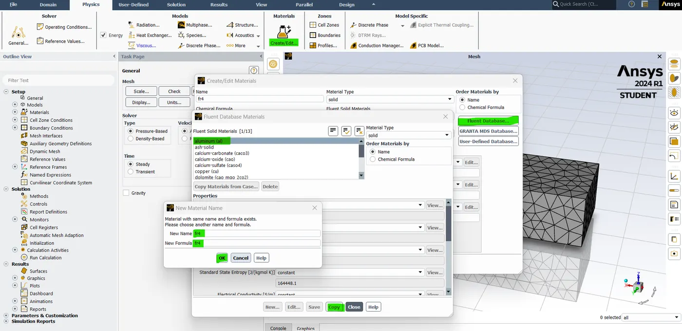
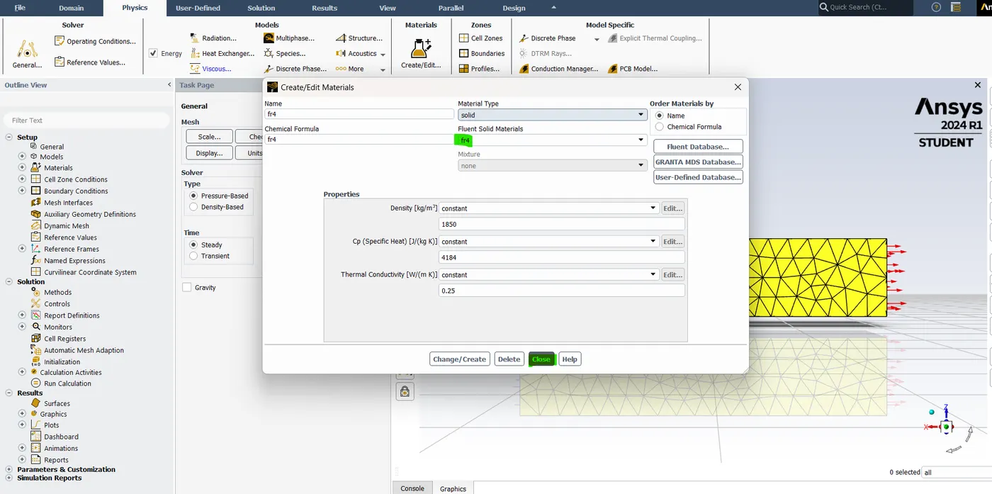
• To create a new material go to fluid database-> select any one material-> change the name of the material and hit "ok"-> and hit copy and close. now change the required material properties and hit change/create. Now the new material "FR4" and its properties are created in solid-type material.

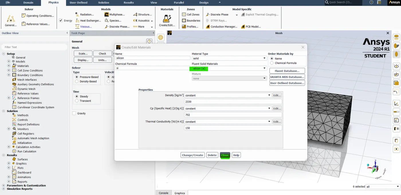
• Similarly create silicon material by changing the name and properties of the material. Now the "Silicon" material is created in solid type material.

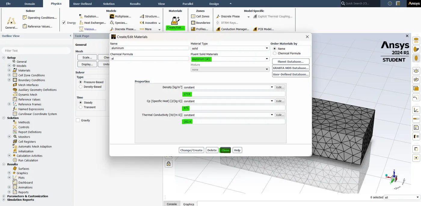
• Similarly create Aluminium material by changing the name and properties of the material. Now the "Aluminium" material is created in solid type material.
• After that now we need to assign the material to the appropriate components. so, go to the cell zones and select the materials.

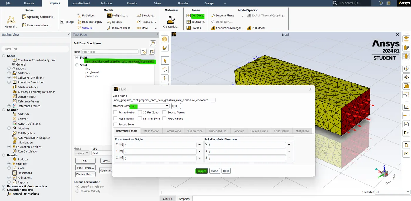
• Go to the cell zones and select the "encloser_encloser" in the Fluid section, then choose the material type as "air" and hit Apply.

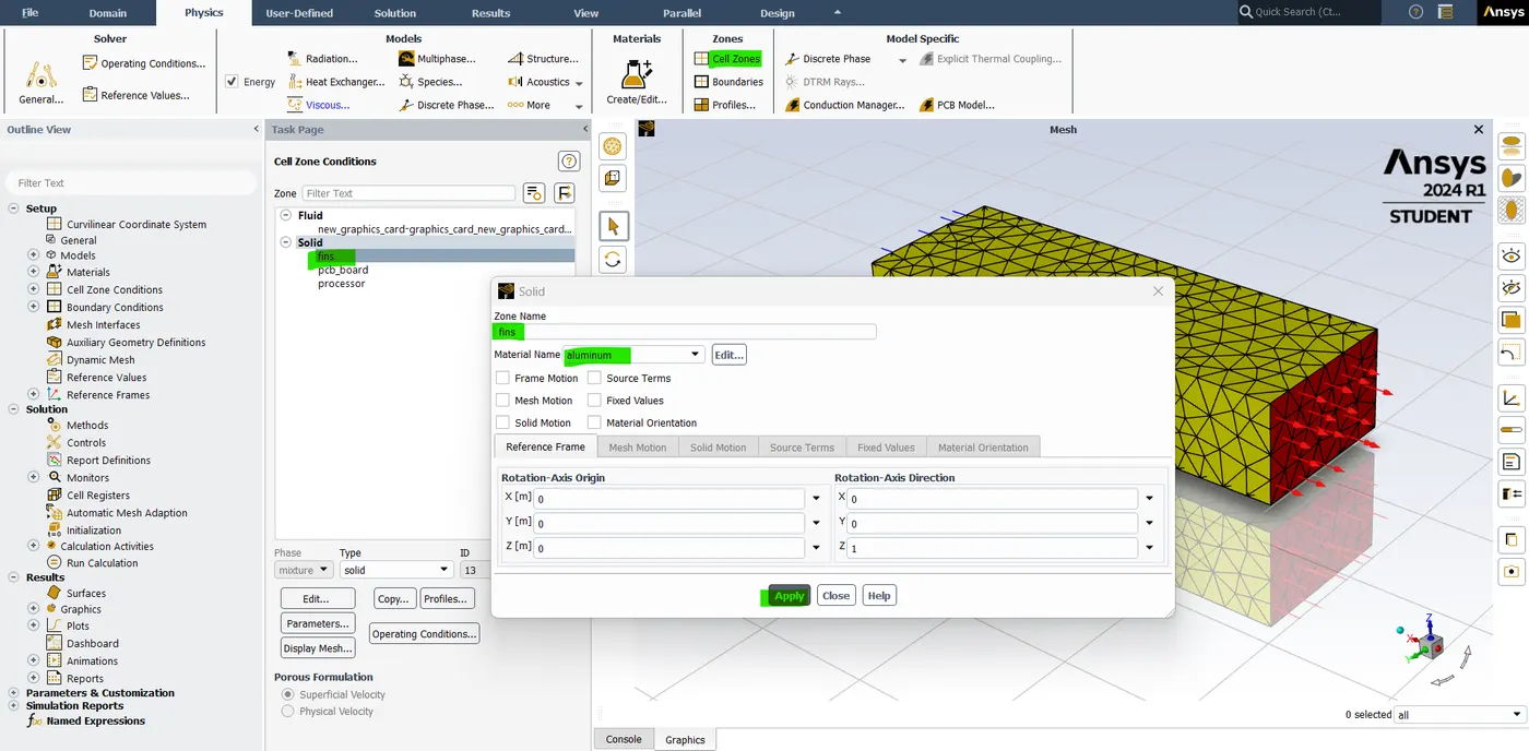
• Go to the cell zones and select the "Fins" in the Solid section, then choose the material type as "Aluminium" and hit Apply.

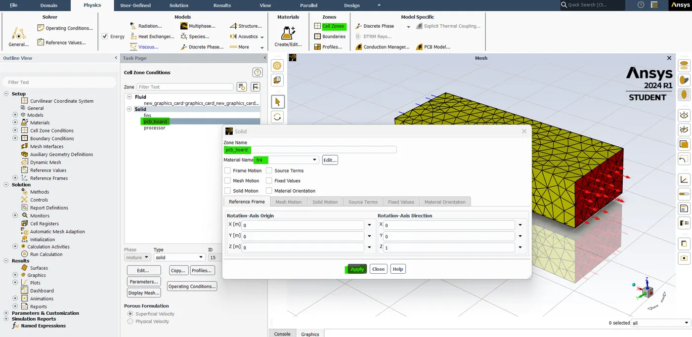
• Go to the cell zones and select the "PCB board" in the Solid section, then choose the material type as "FR4" and hit Apply.

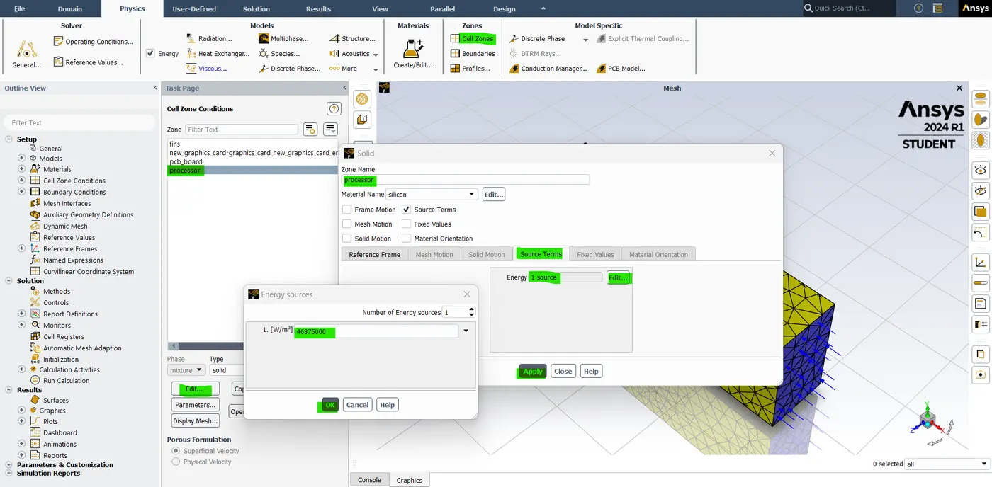
• Go to the cell zones and select the "Processor" in the Solid section, then choose the material type as "Silicon" and then enable the source term by checking the tick box.
• Here, the processor is the heat source from where the heat is being generated. so, select the processor as the source term and give the required value for power density which was calculated before.
• Now go to source term click edit enter the energy source as 1 and then enter the power density value as 46875000 and then hit Apply.
• Now the materials are assigned correctly to the appropriate components. now next we need to create the definition plots.

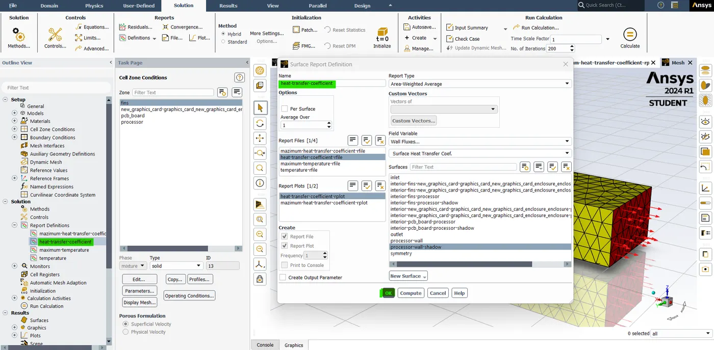
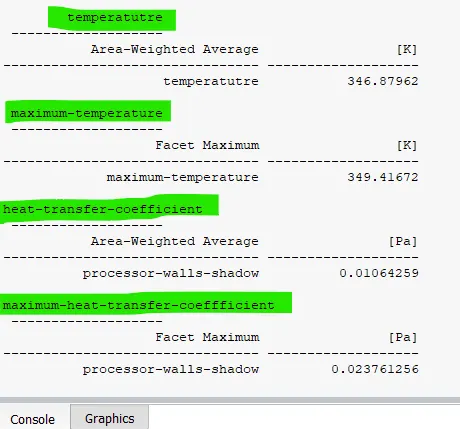
• Now go to Definition and then select the surface report in that select "Area weighted average" and then select the wall Fluxes and surface heat transfer coefficient as a "field variable". Select the "graphics card processor solid" on the surface.
• Name this plot as a "heat transfer coefficient" Hit Apply. Now the HTC definition plot is created.

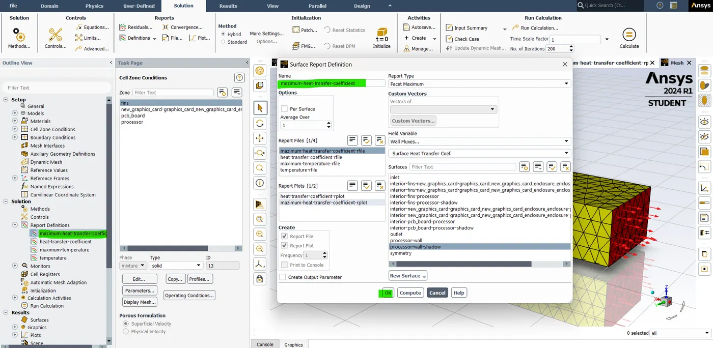
• Now go to Definition and then select the surface report in that select "Facet Maximum" and then select the wall Fluxes and surface heat transfer coefficient as a "field variable". Select the "processor" on the surface.
• Name this plot as a "Maximum heat transfer coefficient" Hit Apply. Now the maximum HTC definition plot is created.

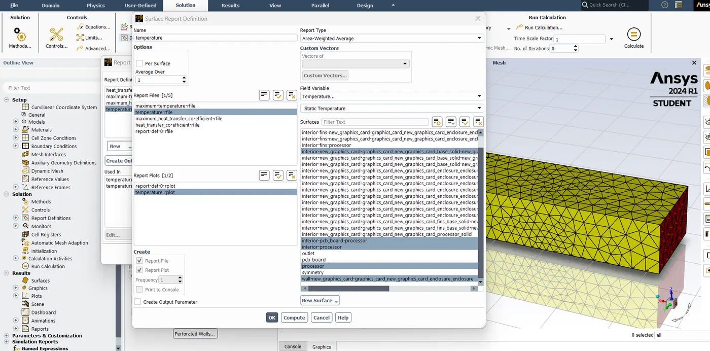
• Now go to Definition and then select the surface report in that select "Area weighted average" and then select the Temperature and static temperature as a "field variable". Select the "processor, interior pcb_board processor, interior processor, interior fins processor, graphics card base solid, graphics card enclosure_enclosure" in the surface.
• Name this plot as a "Temperature" Hit Apply. Now the Temperature definition plot is created.

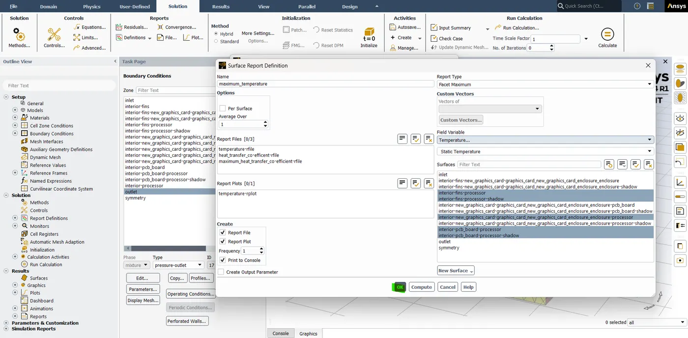
• Now go to Definition and then select the surface report in that select "Facelet maximum" and then select the Temperature and static temperature as a "field variable". Select the "processor, interior pcb_board processor, interior processor, interior fins processor, graphics card base solid, graphics card enclosure_enclosure" in the surface.
• Name this plot as a "Maximum Temperature" Hit Apply. Now the Temperature definition plot is created.
• After that now initialize the simulation. so, hit hybrid initialization.

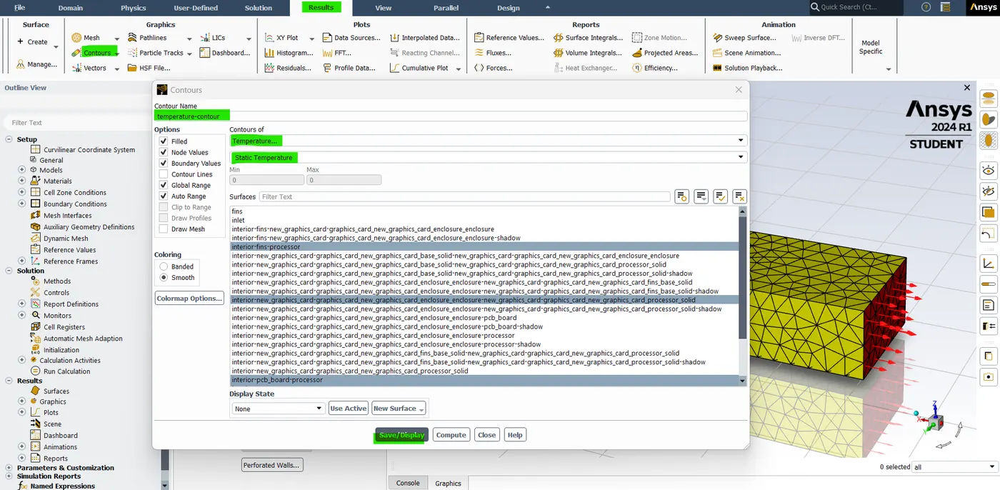
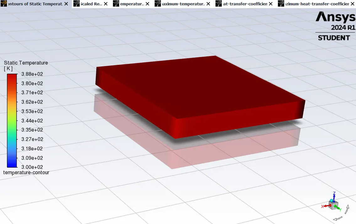
• Now to see the temperature changes we need to create the temperature contour plot. so go to contour plot and then select the "temperature and static temperature" in contour type and select the "interior fins processor, interior PCB board processor, graphics card eneclosure_enclosure processor solid" and hit save/display.

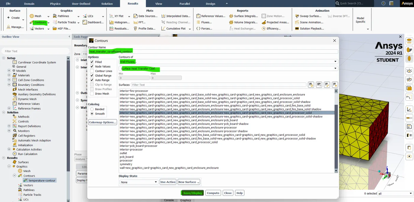
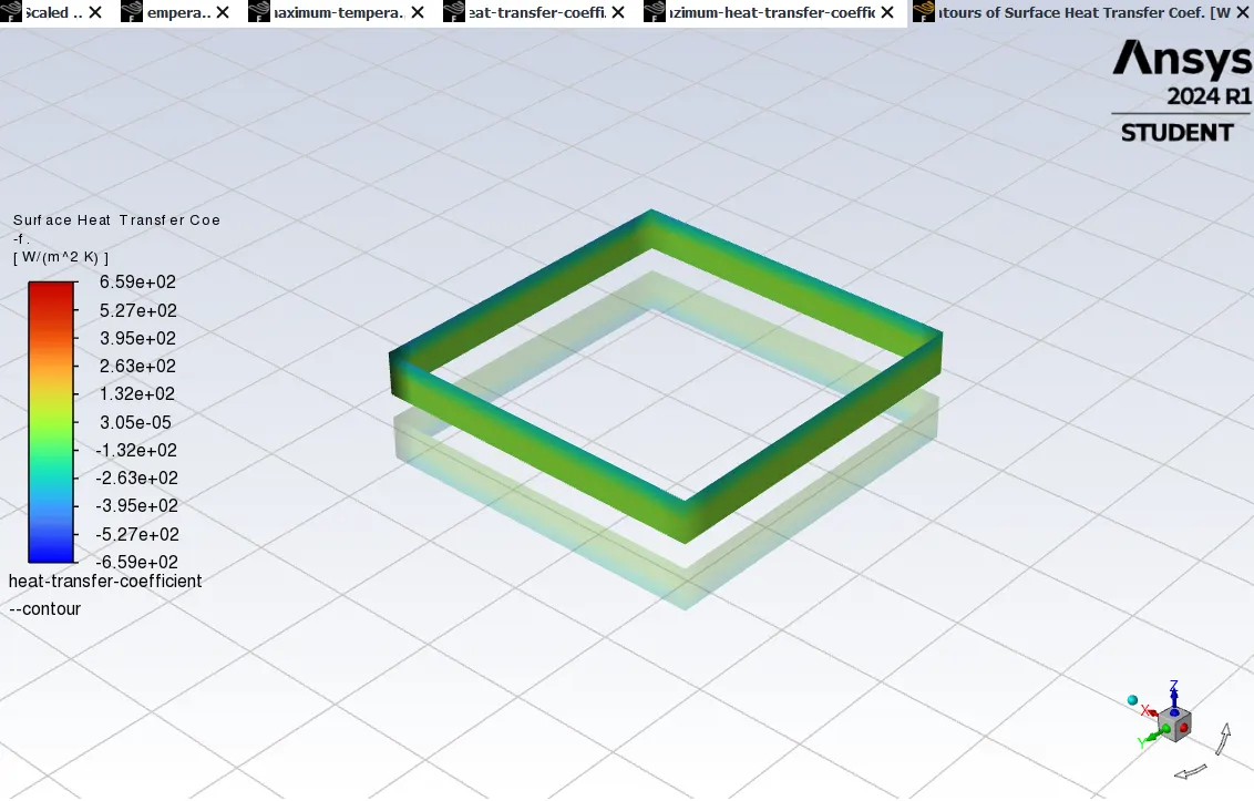
• Now to see the temperature changes we need to create the temperature contour plot. so go to contour plot and then select the "wall and surface heat transfer coefficient" in contour type and select the "interior fins processor, interior PCB board processor, graphics card eneclosure_enclosure processor solid" and hit save/display.

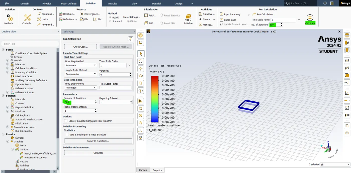
• Once hybrid initialization is done. Now finally we need to give no.of. iterations is 500. Hit calculate to run the simulation.

Result:

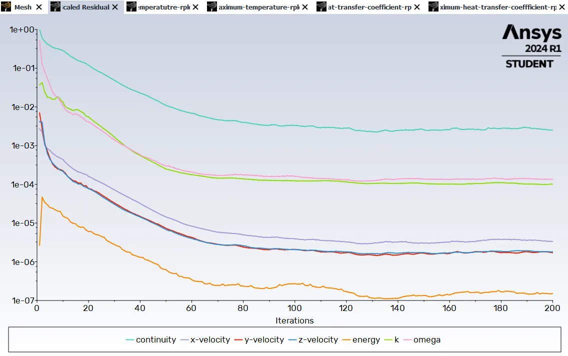
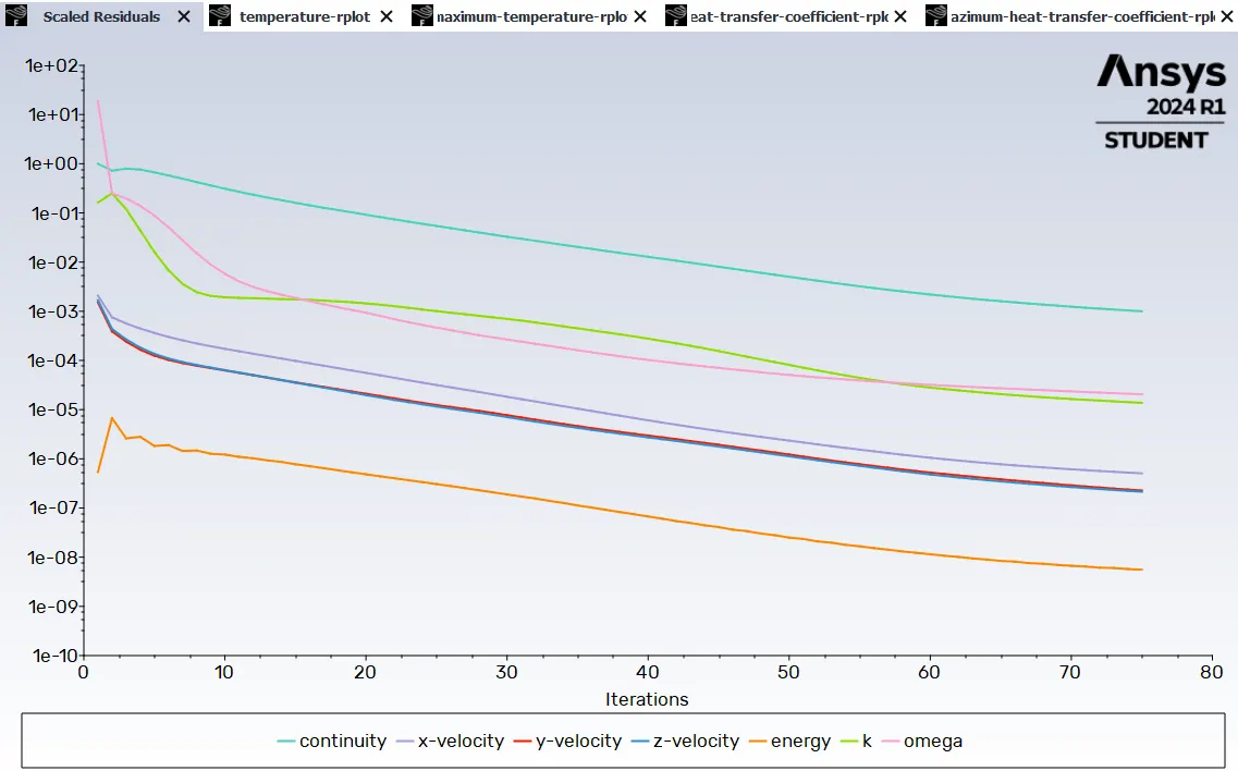
Residuals plot:

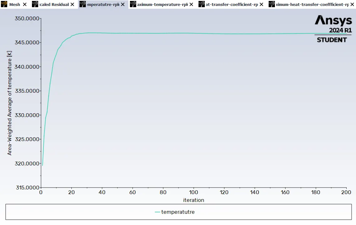
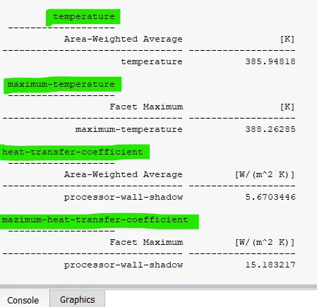
Average Temperature plot (processor):

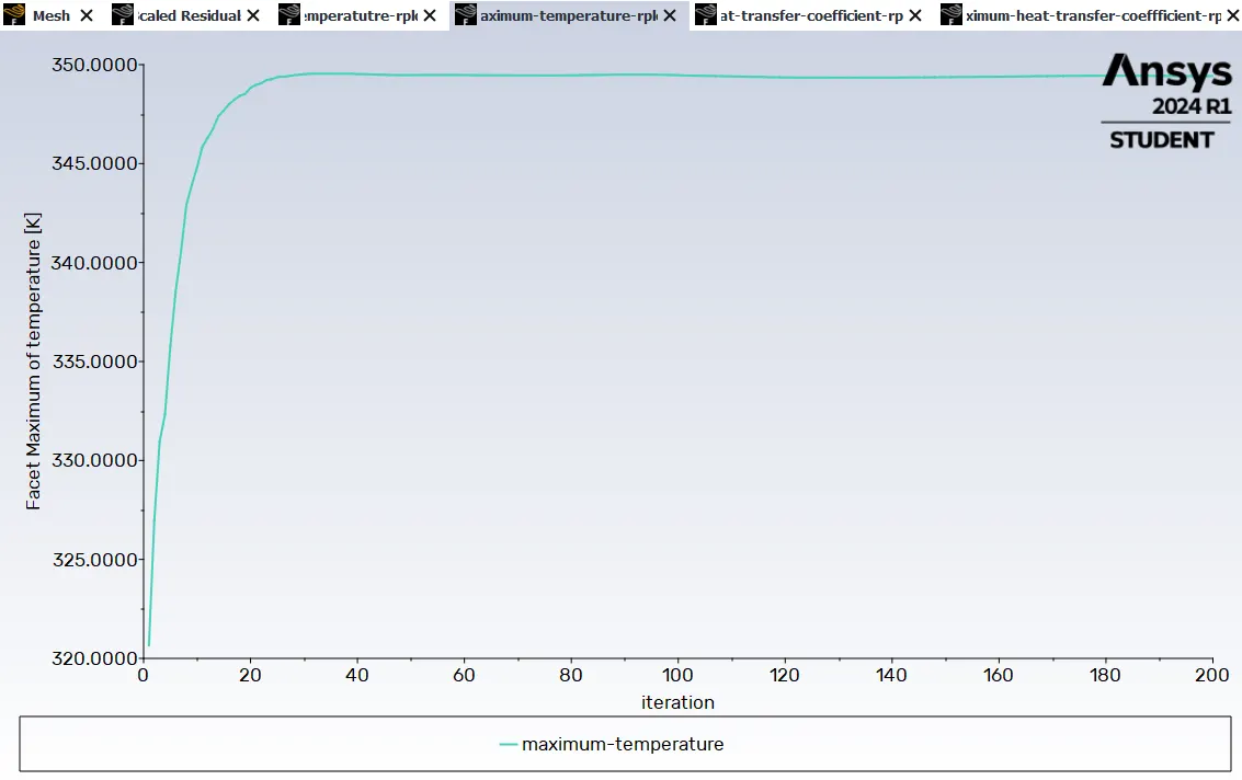
Maximum Temperature Plot (processor):

Average Heat transfer coefficient (processor):

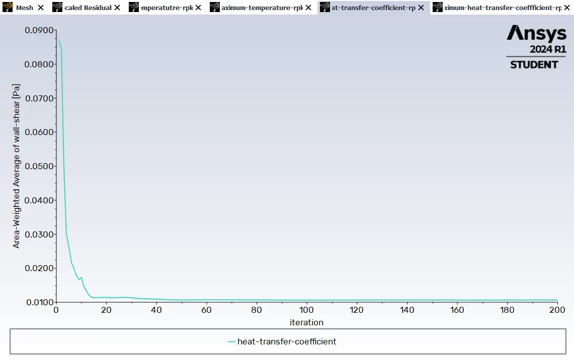
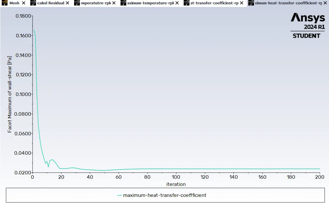
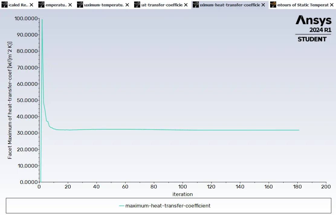
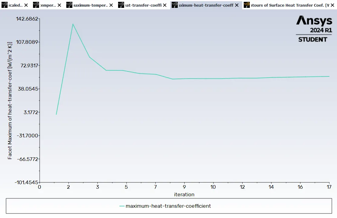
Maximum Heat transfer coefficient (processor):

Post processor:

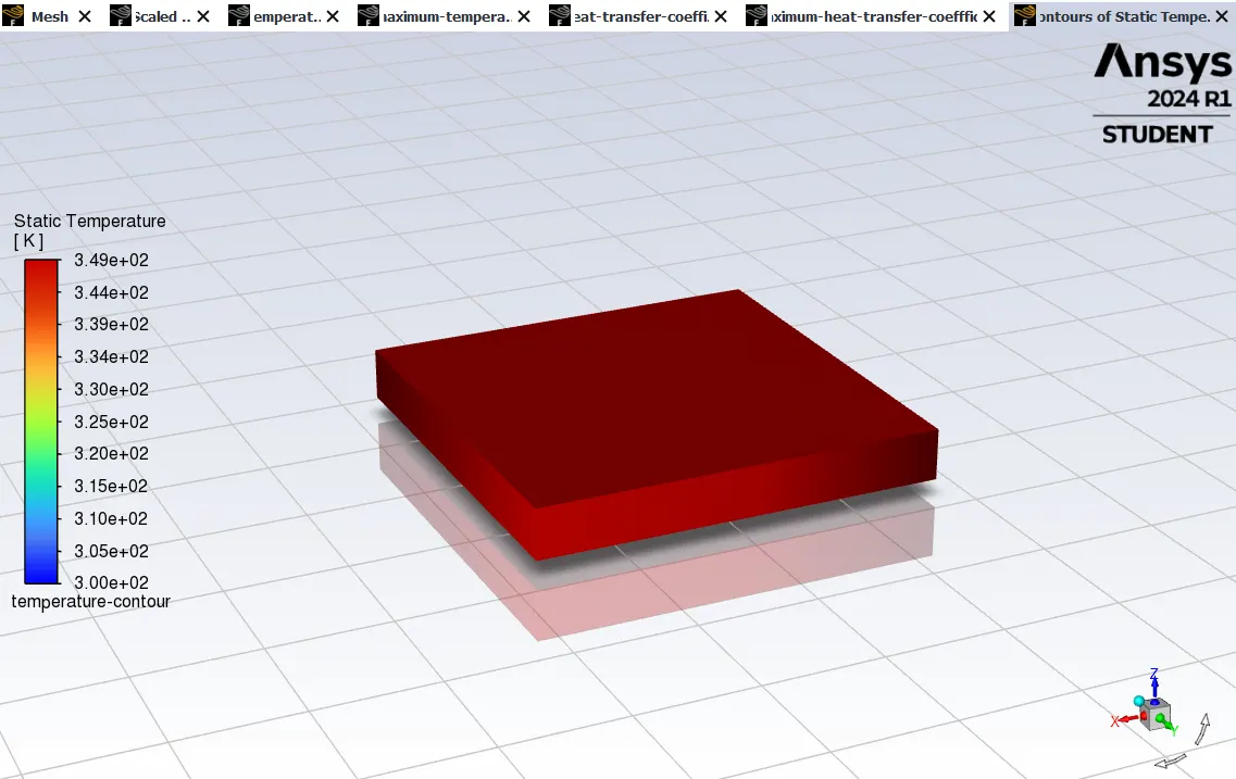
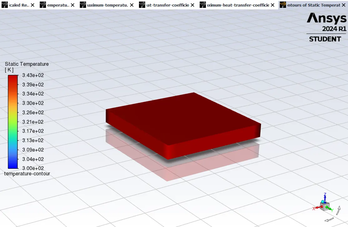
Temperature contour (Processor):

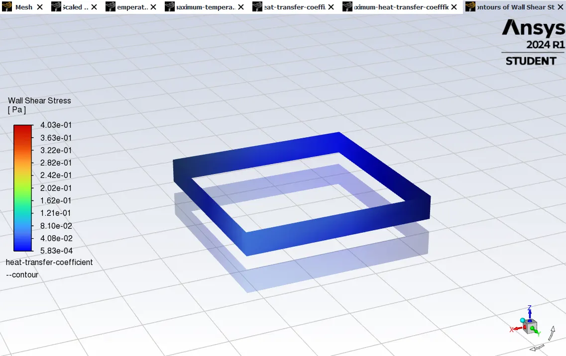
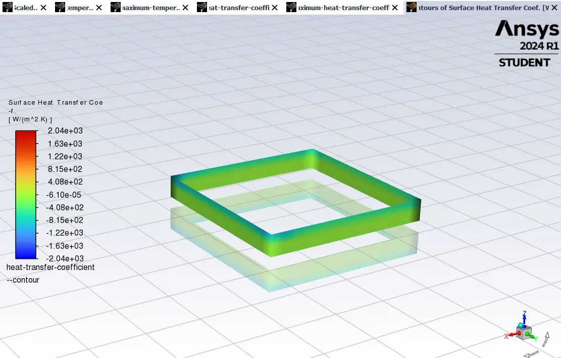
Heat transfer co-efficient contour (Processor):

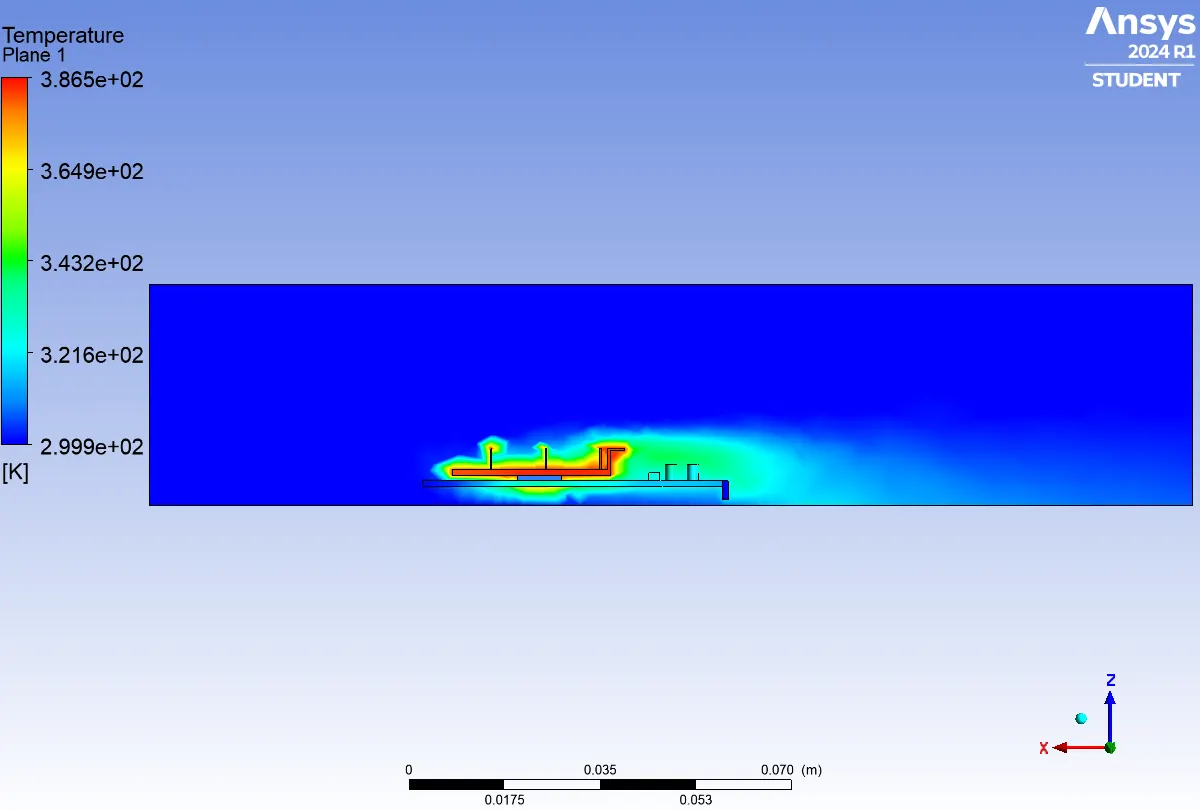
Temperature contour (XZ plane):

Velocity contour (XZ plane):

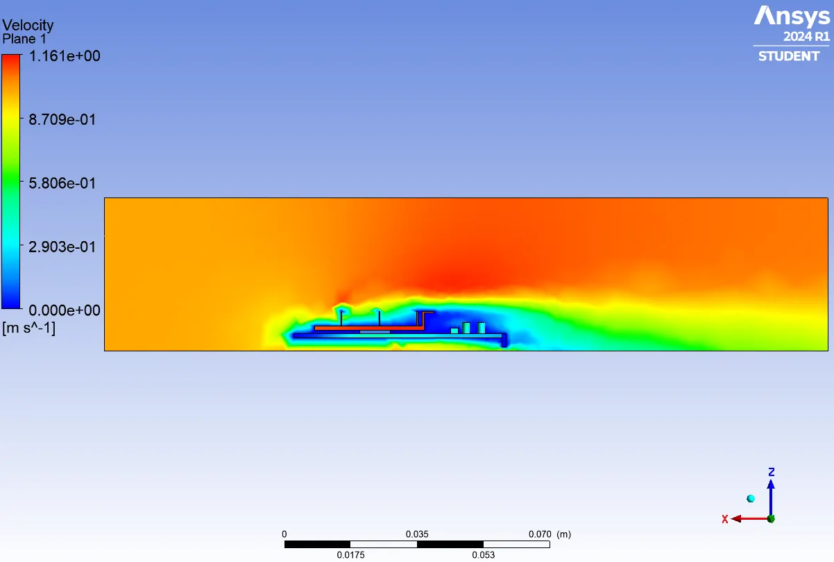
velocity vector (XZ Plane):

Temperature contour (fins, processor, PCB):

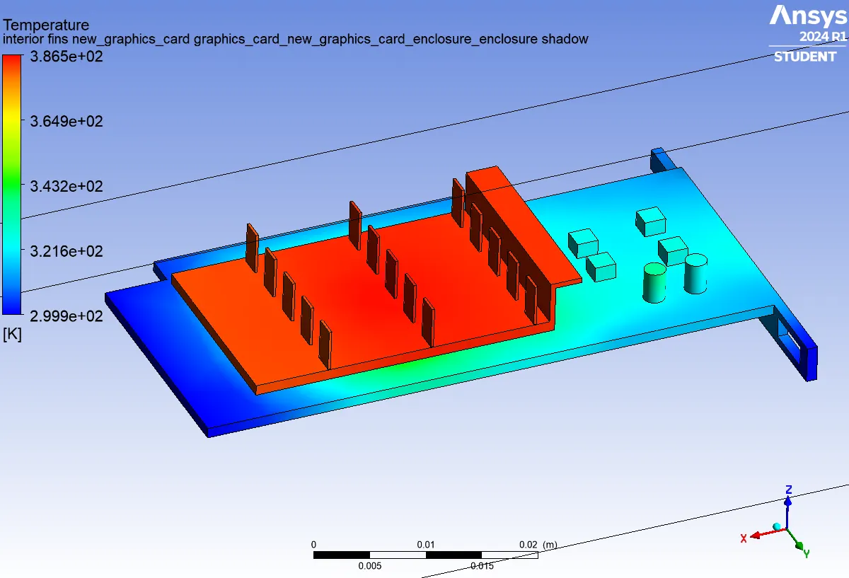
Case-2 (Refined mesh, v=1 m/s)

Meshing & Solving approach:-

• In this case the geomentry are same which we followed in the baseline mesh. After that, we moved towards the meshing module. so, here we need to create the meshing specifically for each component. So, that will help to change the mesh size in a specific area.

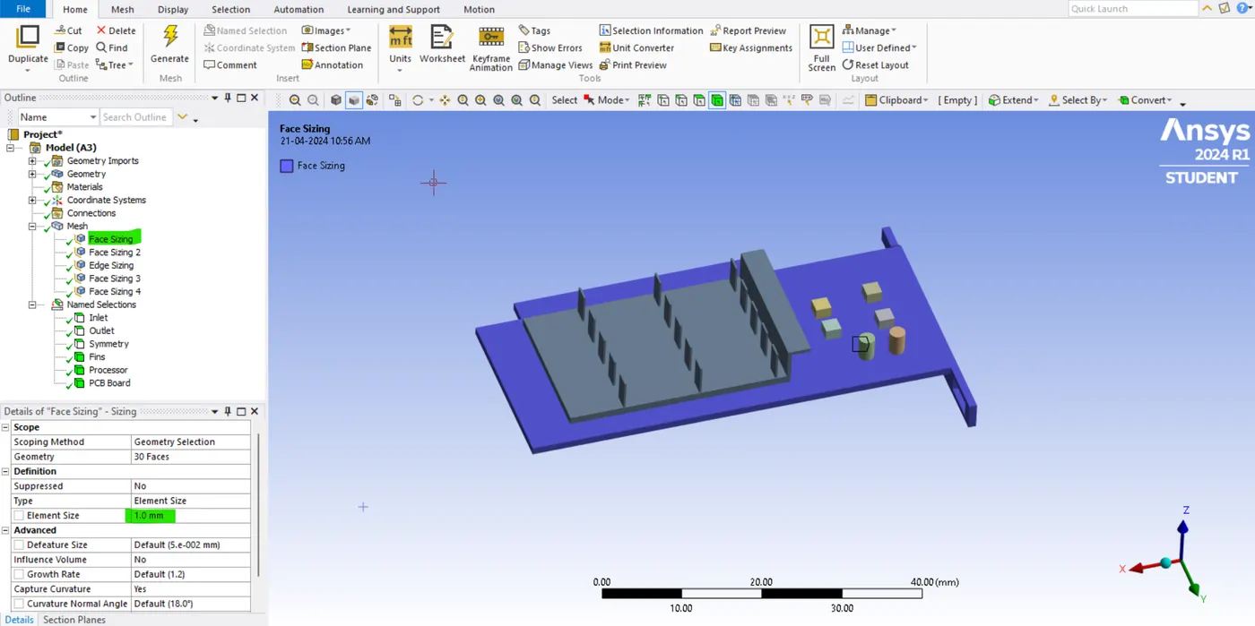
• Add the face sizing for the PCB board and the PCB board mesh element size is 1 mm.

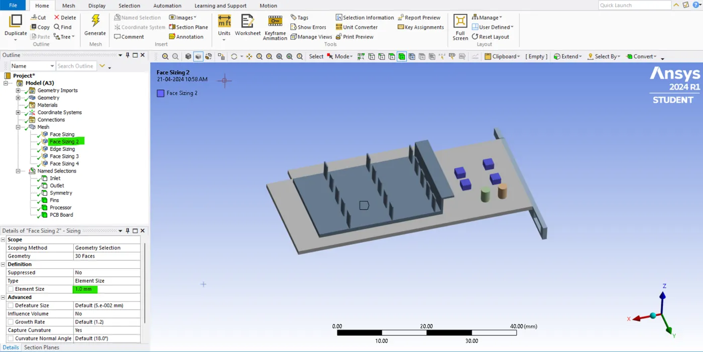
• Add the face sizing for the four cube processors and the processor mesh element size is 1 mm.

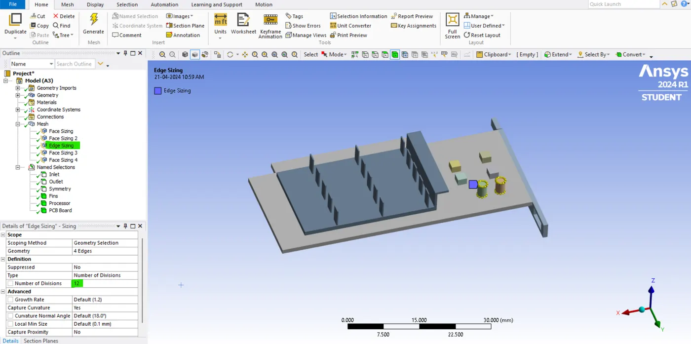
• Add the edge sizing for the cylinder and the cylinder no.of.division is 12. The mesh element size is 1 mm.

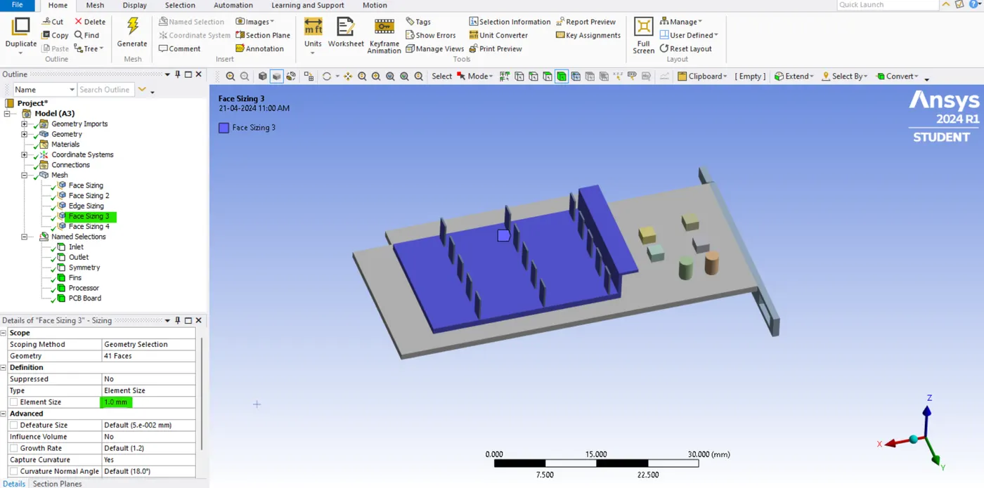
• Add the face sizing for the fins and the fins mesh element size is 1 mm. Here we need to select fins except the fins tip.

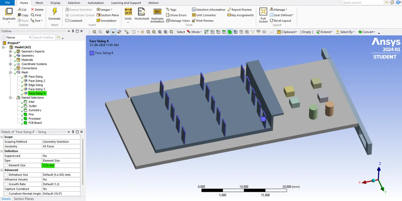
• Add the face sizing for the fins tip and the fins tip mesh element size is 0.25 mm.

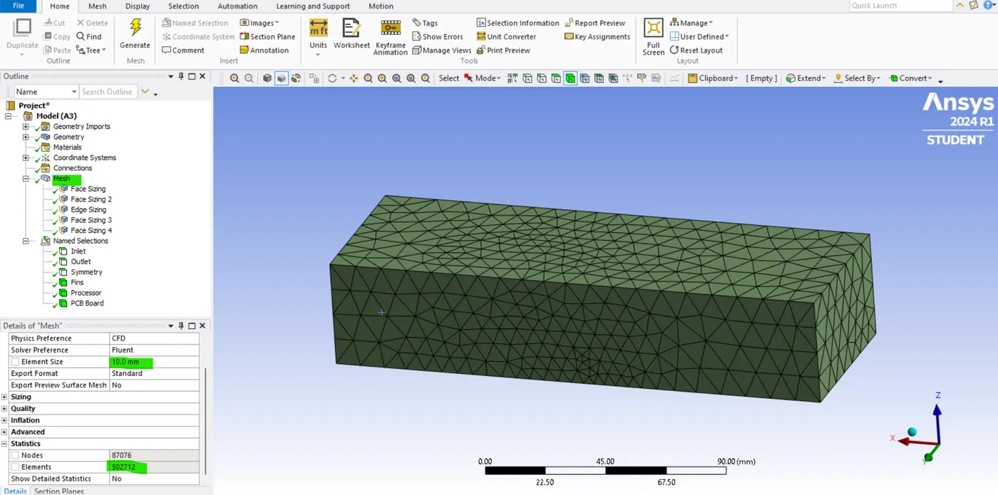
• For Enclosure the mesh element size is 10 mm. And the total no.of.mesh element is 502712.

PCB Board:

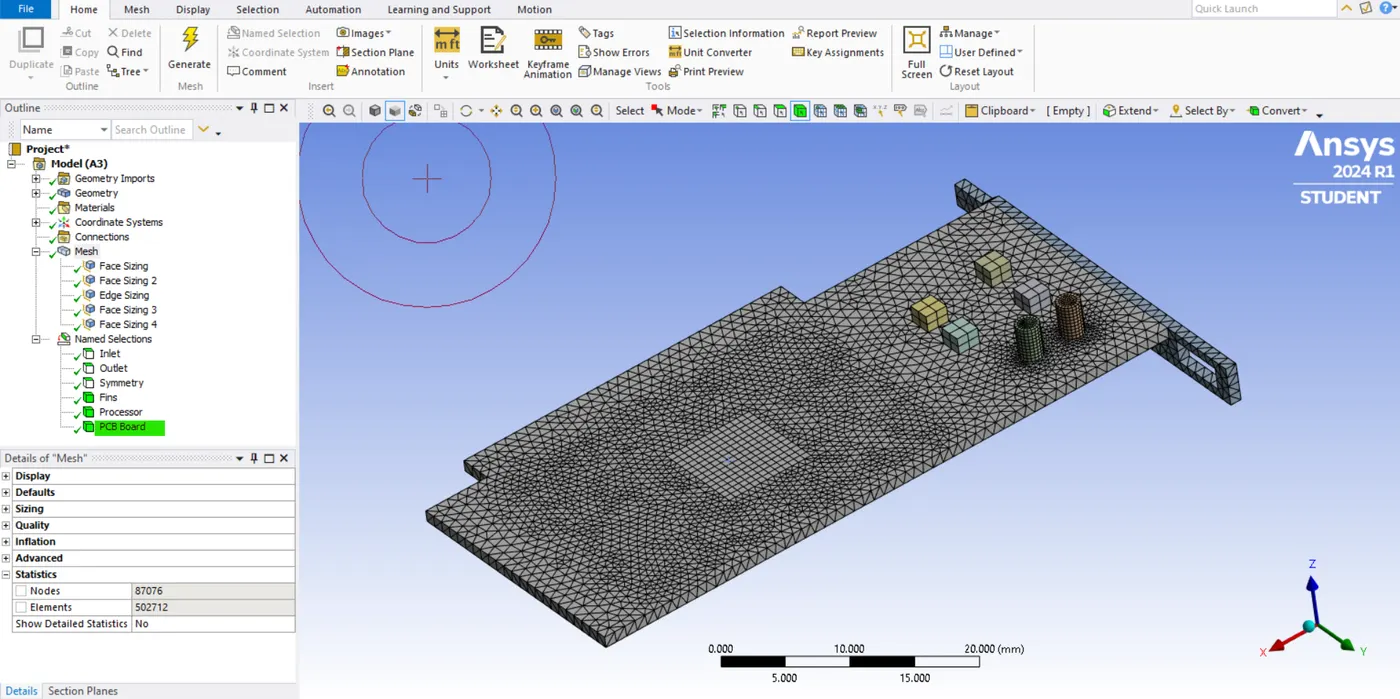
• After updating the PCB Board meshing, it will look like this.

Fins:

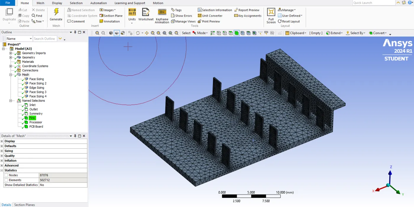
• After updating the Fins meshing, it will look like this.

Processor:

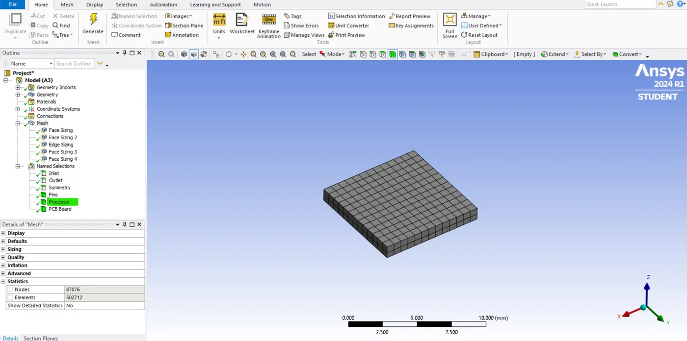
• After updating the Processor meshing, it will look like this.

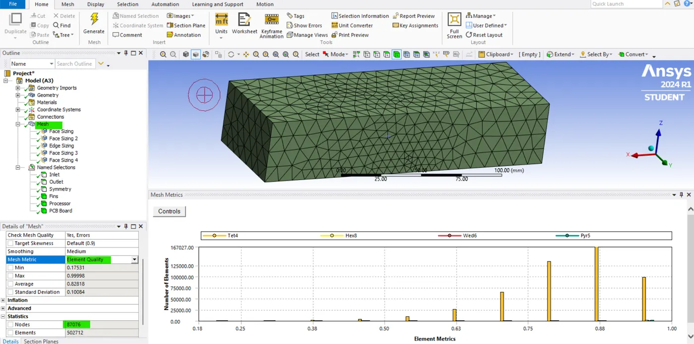
• The total no.of.mesh is 87076. And also you can see the mesh metric.

Setup & modeling approach:-

• Now we need to add new materials for different components in the material list by copying one material's properties and naming them as other materials.

• Now go to create material and then select "air" material in fluid material type. After that hit apply.

• To create a new material go to fluid database-> select any one material-> change the name of the material and hit "ok"-> and hit copy and close. now change the required material properties and hit change/create. Now the new material "FR4" and its properties are created in solid-type material.

• Similarly create silicon material by changing the name and properties of the material. Now the "Silicon" material is created in solid type material.

• Similarly create Aluminium material by changing the name and properties of the material. Now the "Aluminium" material is created in solid type material.

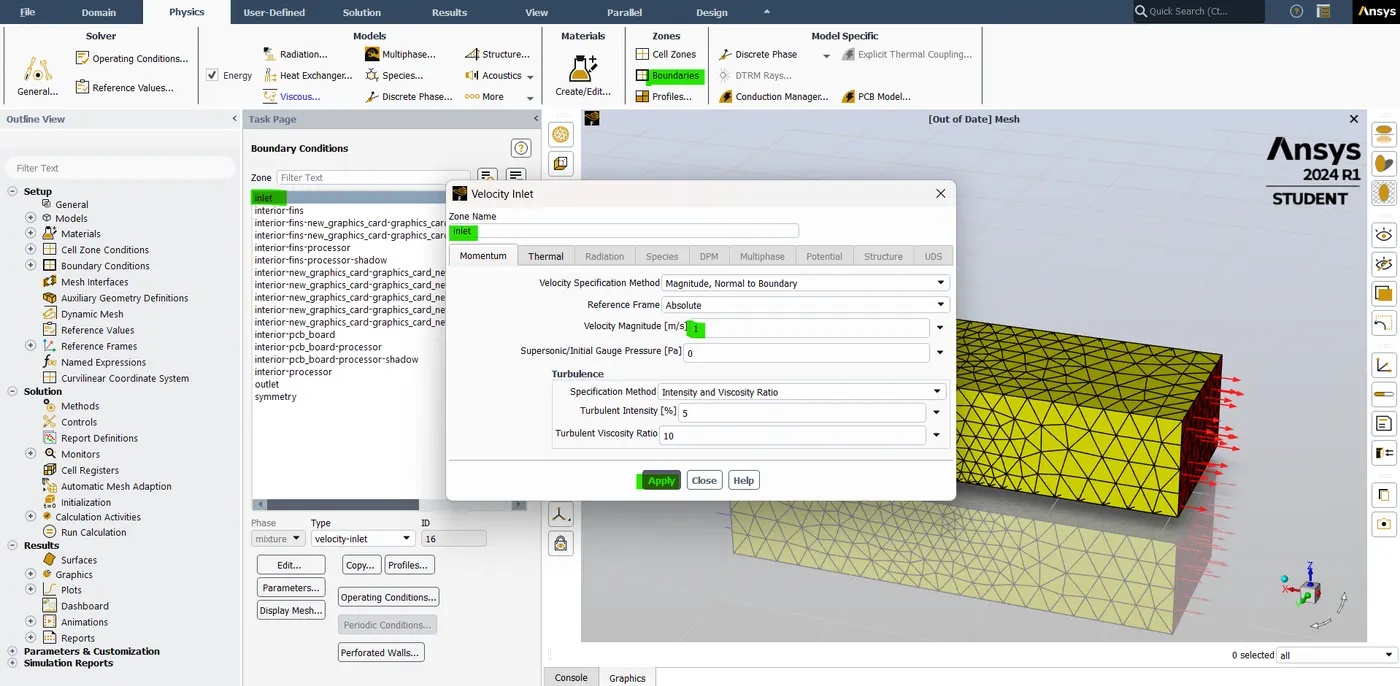
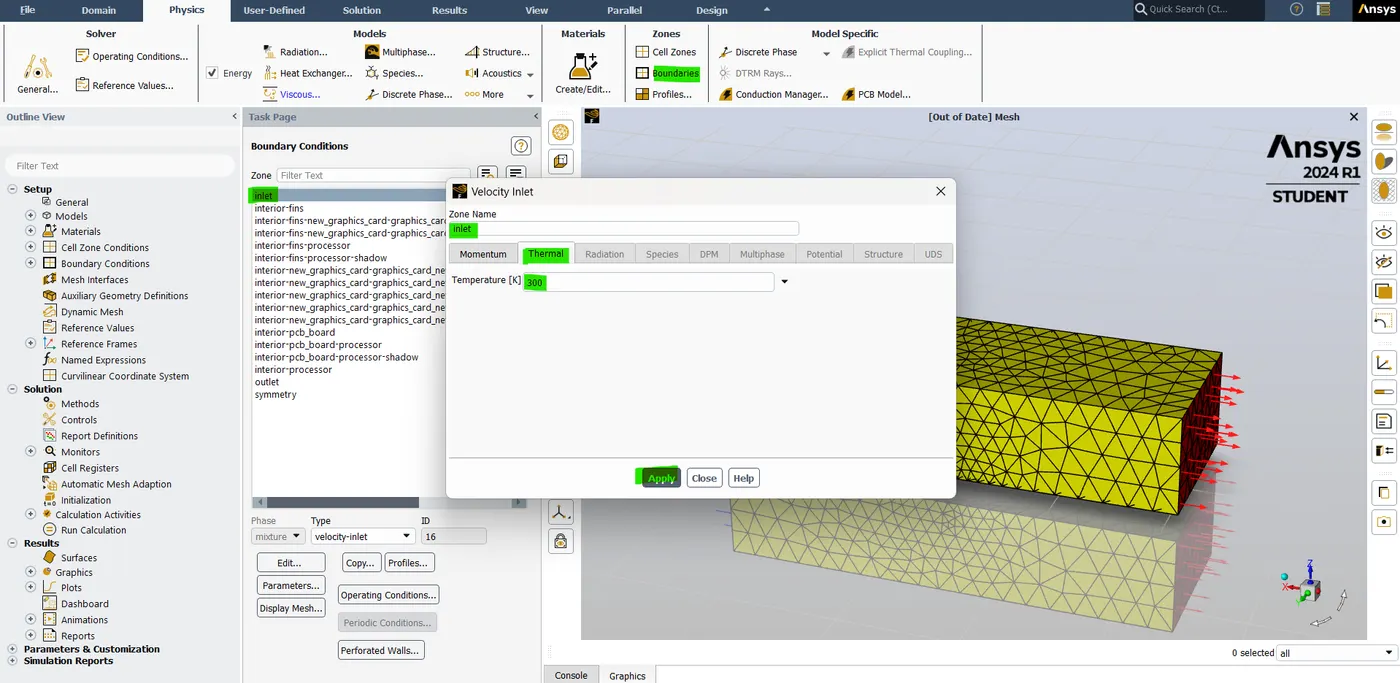
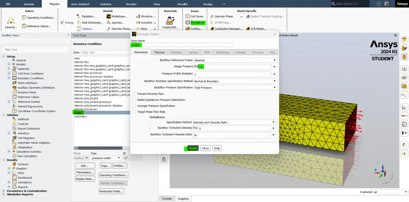
• Here assign the boundary conditions for Inlet is 3m/s, temperature is 300 K and the outlet is 0m/s. And then hit apply. now next we need to create the definition plots.

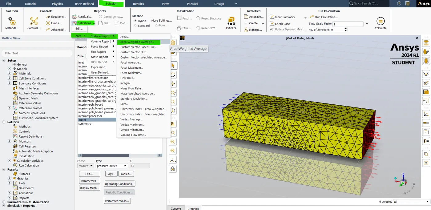
• Now go to Definition and then select the surface report in that select "Area weighted average" and then select the wall Fluxes and surface heat transfer coefficient as a "field variable". Select the "graphics card processor solid" on the surface.
• Name this plot as a "heat transfer coefficient" Hit Apply. Now the HTC definition plot is created.

• Now go to Definition and then select the surface report in that select "Facet Maximum" and then select the wall Fluxes and surface heat transfer coefficient as a "field variable". Select the "processor" on the surface.
• Name this plot as a "Maximum heat transfer coefficient" Hit Apply. Now the maximum HTC definition plot is created.

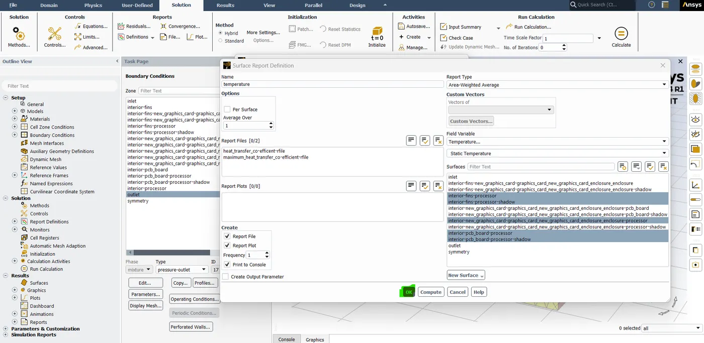
• Now go to Definition and then select the surface report in that select "Area weighted average" and then select the Temperature and static temperature as a "field variable". Select the "processor, interior pcb_board processor, interior processor, interior fins processor, graphics card base solid, graphics card enclosure_enclosure" in the surface.
• Name this plot as a "Temperature" Hit Apply. Now the Temperature definition plot is created.

• Now go to Definition and then select the surface report in that select "Facelet maximum" and then select the Temperature and static temperature as a "field variable". Select the "processor, interior pcb_board processor, interior processor, interior fins processor, graphics card base solid, graphics card enclosure_enclosure" in the surface.
• Name this plot as a "Maximum Temperature" Hit Apply. Now the Temperature definition plot is created.

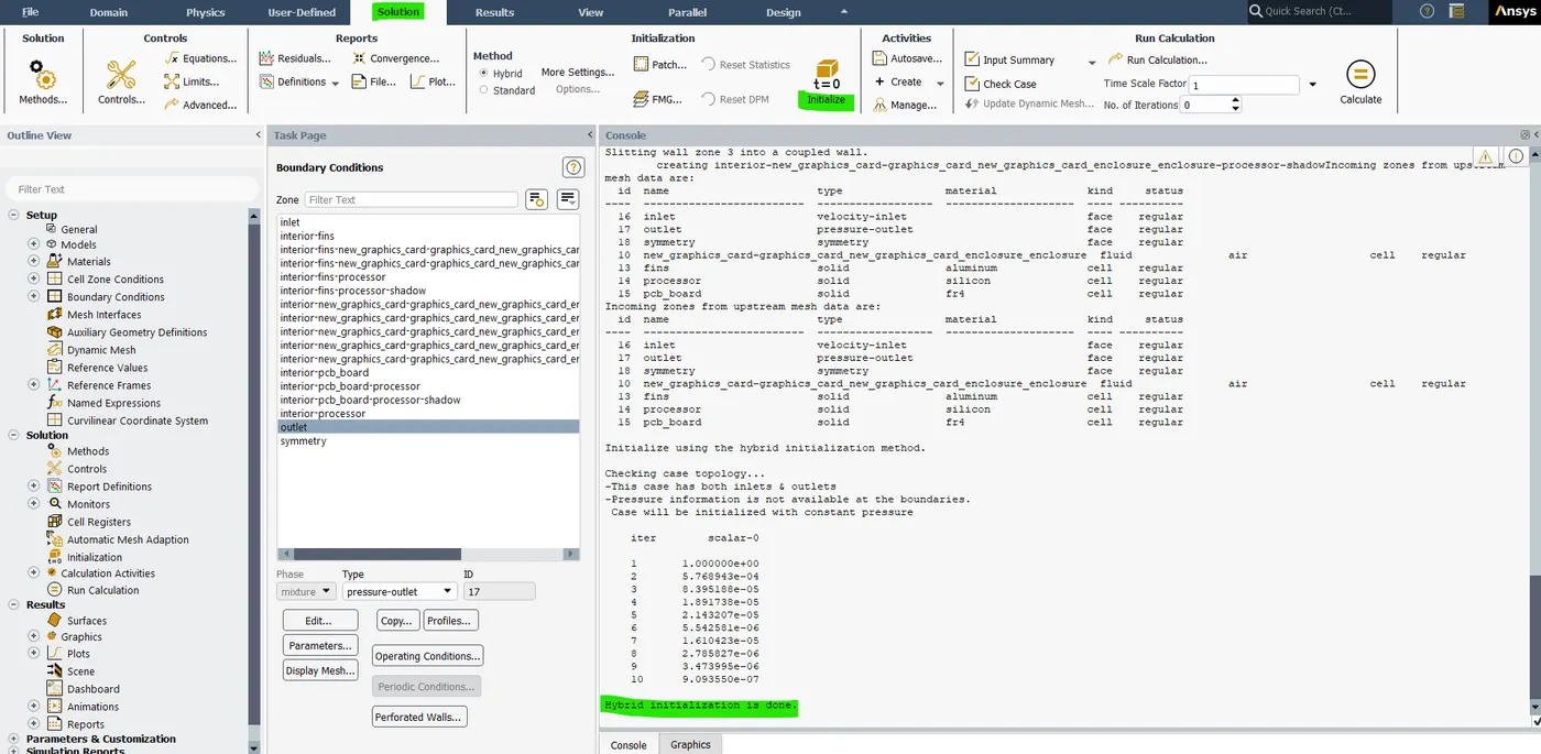
• After that now initialize the simulation. so, hit hybrid initialization.

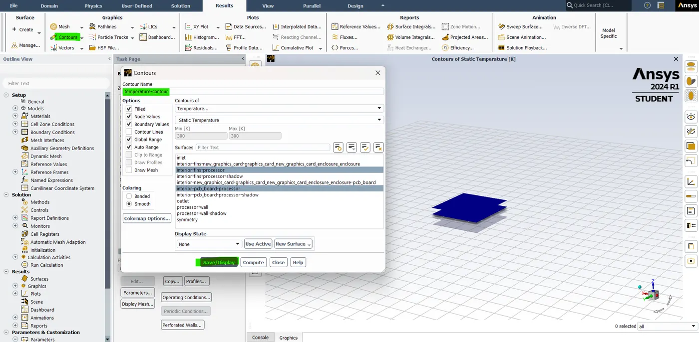
• Now to see the temperature changes we need to create the temperature contour plot. so go to contour plot and then select the "temperature and static temperature" in contour type and select the "interior fins processor, interior PCB board processor, graphics card eneclosure_enclosure processor solid" and hit save/display.

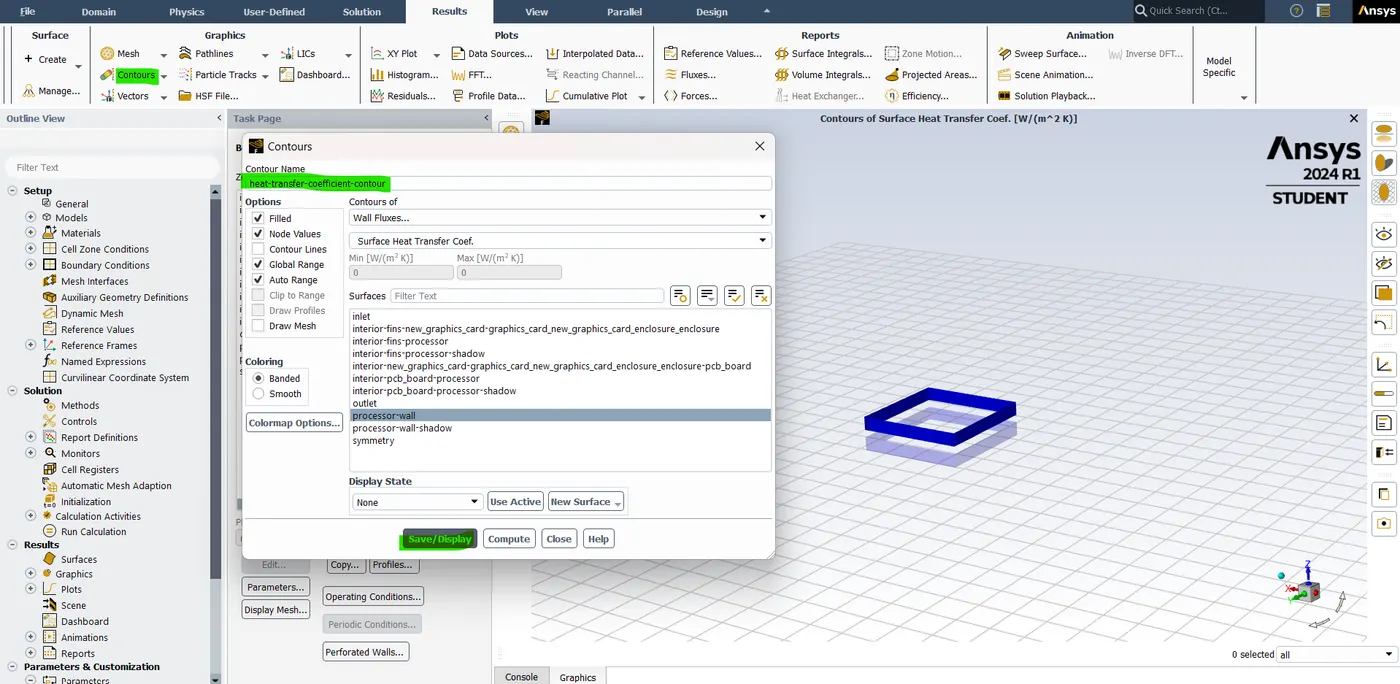
• Now to see the temperature changes we need to create the temperature contour plot. so go to contour plot and then select the "Wall Fluxes and surface heat transfer coefficient" in contour type and select the "new graphics card eneclosure_enclosure graphics card processor solid" and hit save/display.

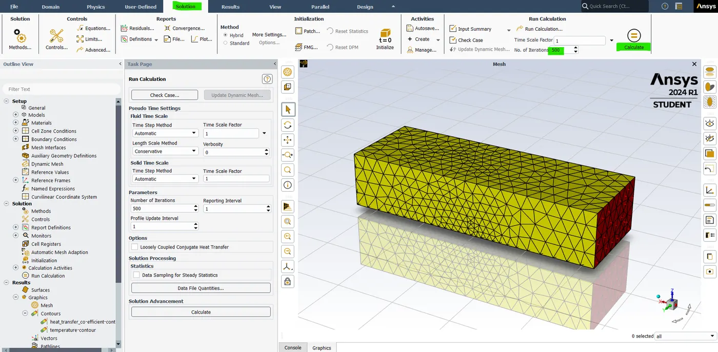
• Once hybrid initialization is done. Now finally we need to give no.of. iterations is 500. Hit calculate to run the simulation.

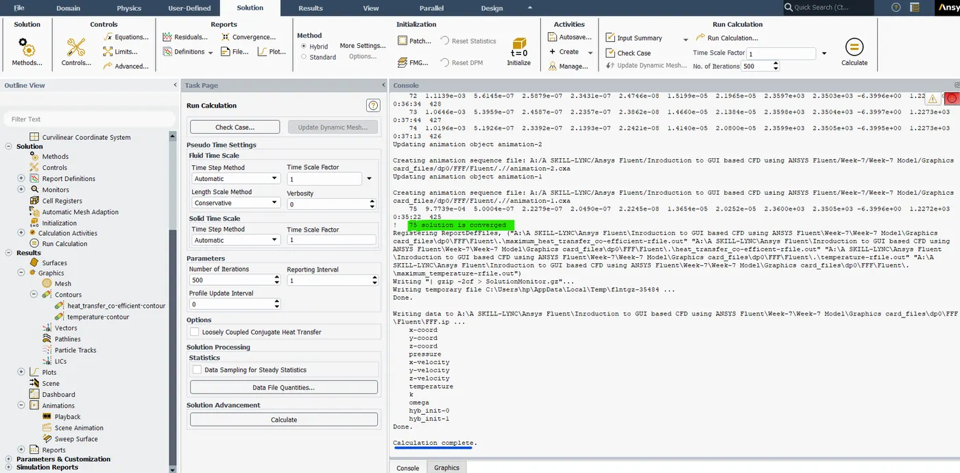
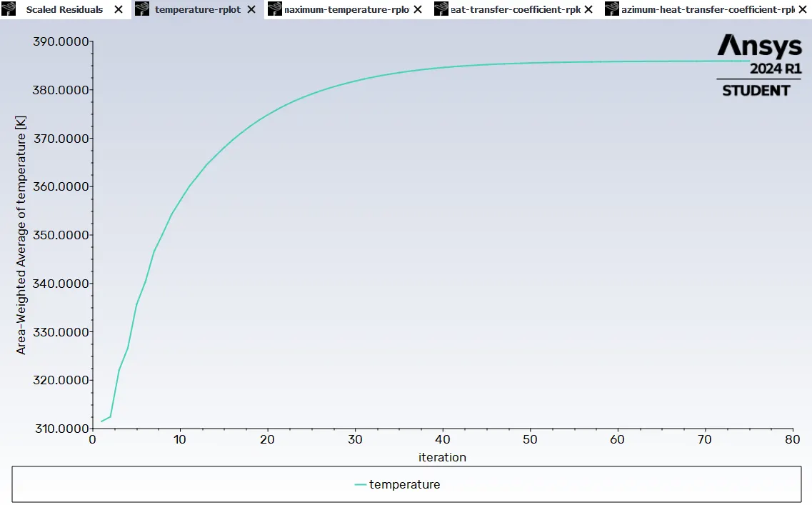
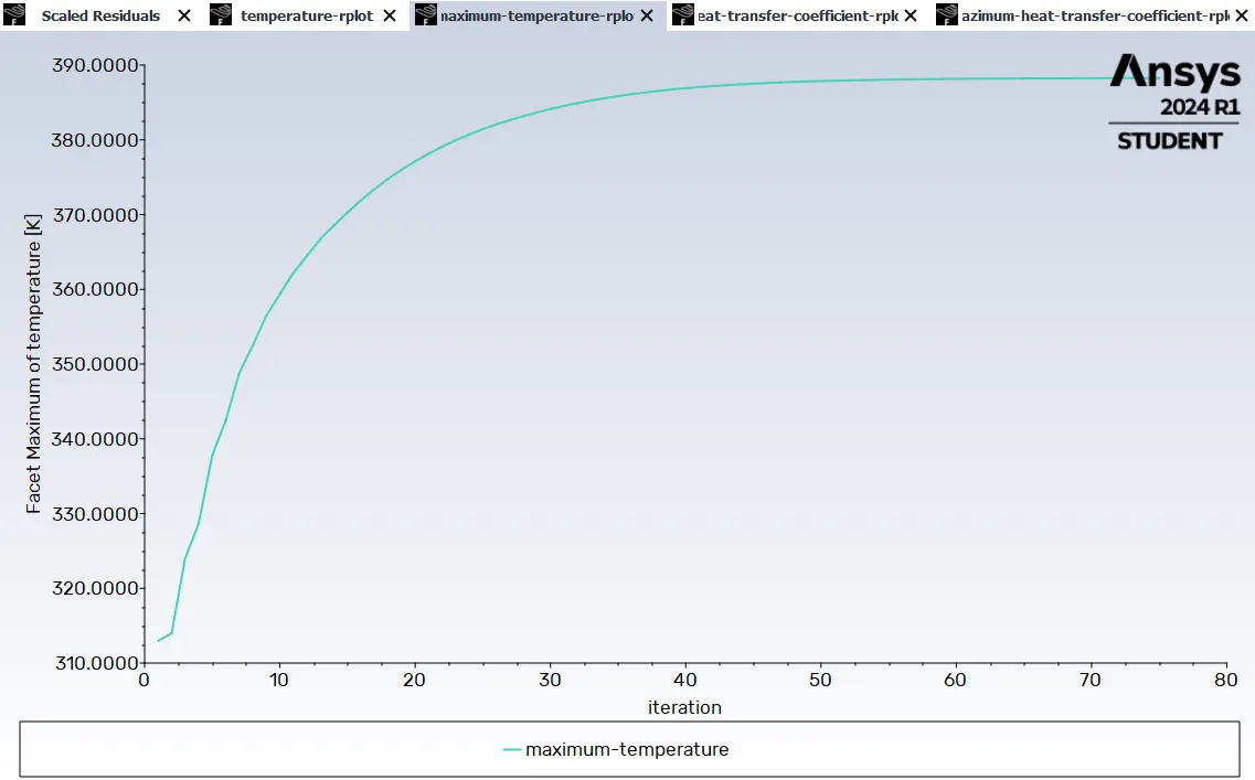
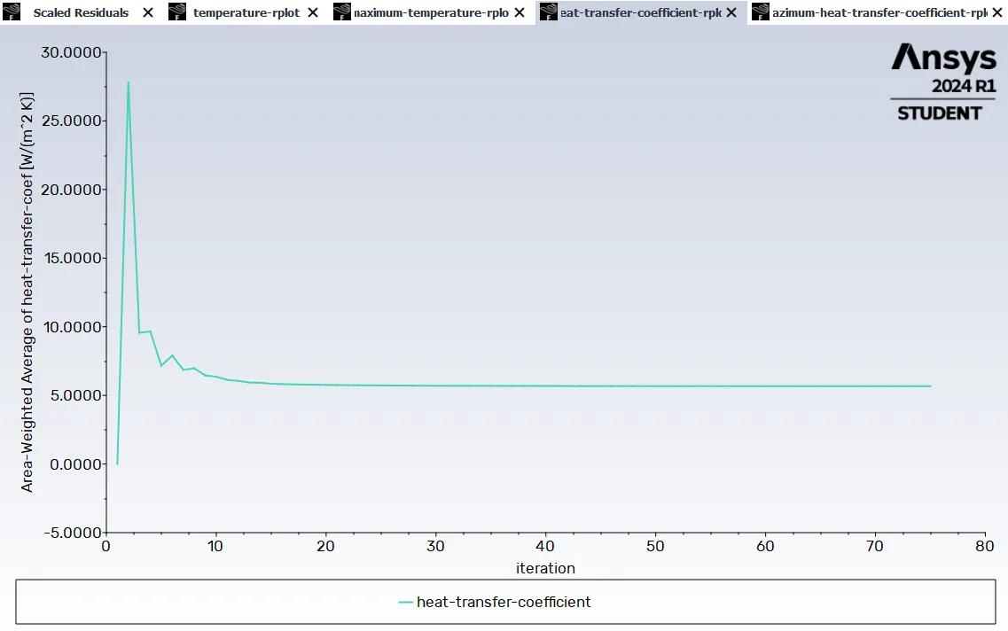
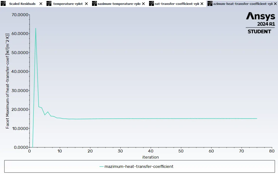
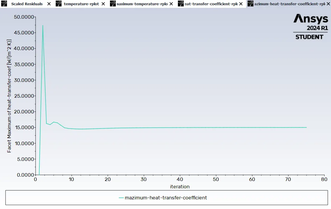
• At the 76^th iteration the solution got converged.

Result:

Residuals plot:

Average Temperature plot (processor):

Maximum Temperature Plot (processor):

Average Heat transfer coefficient (processor):

Maximum Heat transfer coefficient (processor):

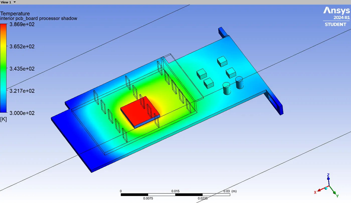
Temperature contour (Processor):-

Heat transfer co-efficient contour (Processor):

Post-processor and solver setting:

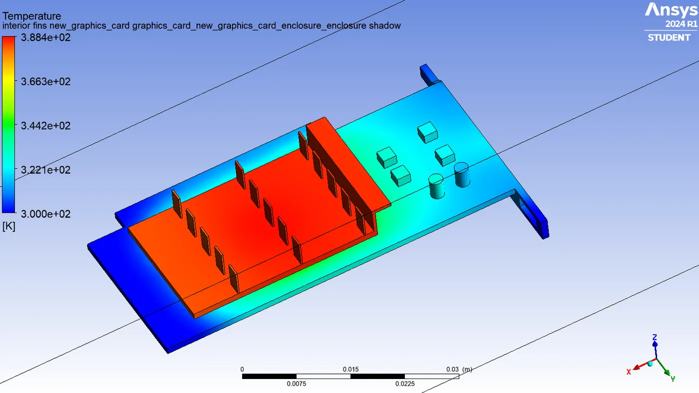
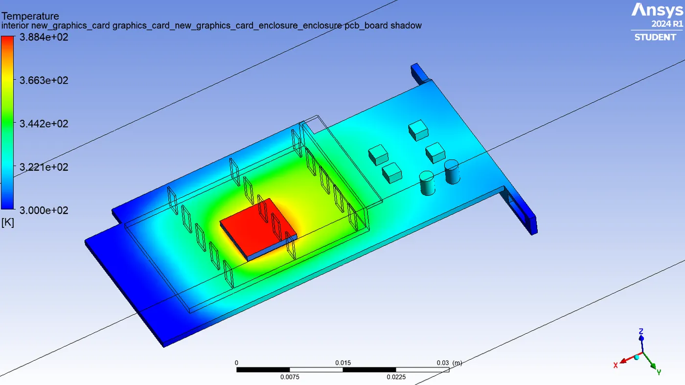
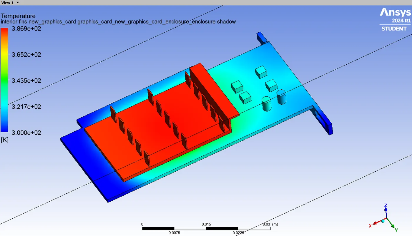
Temperature contour (fins, processor, PCB):

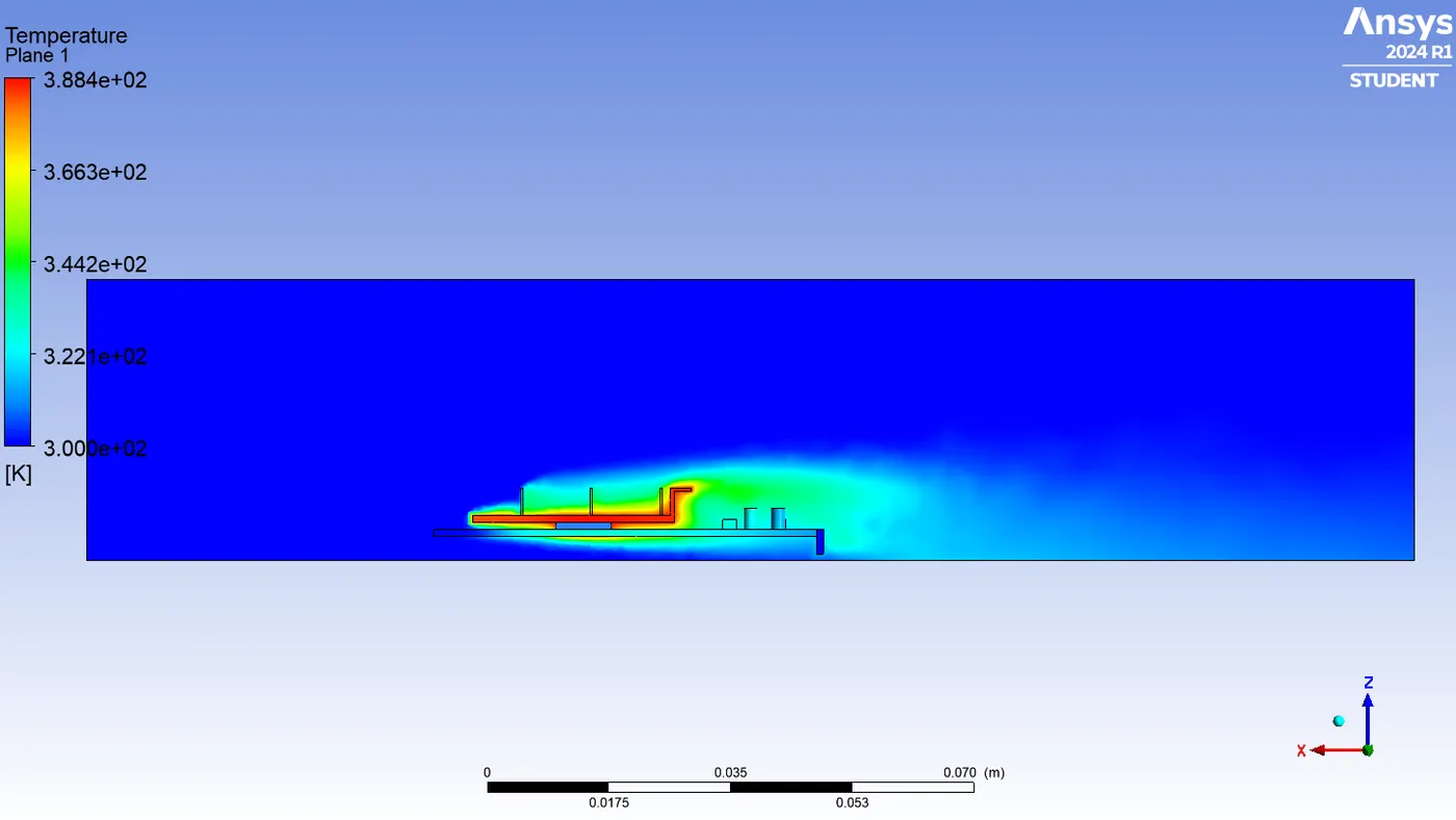
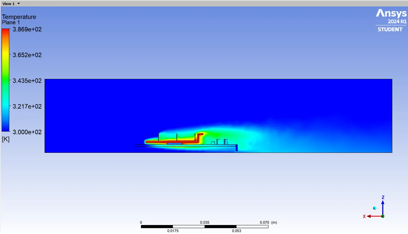
Temperature contour (XZ plane):

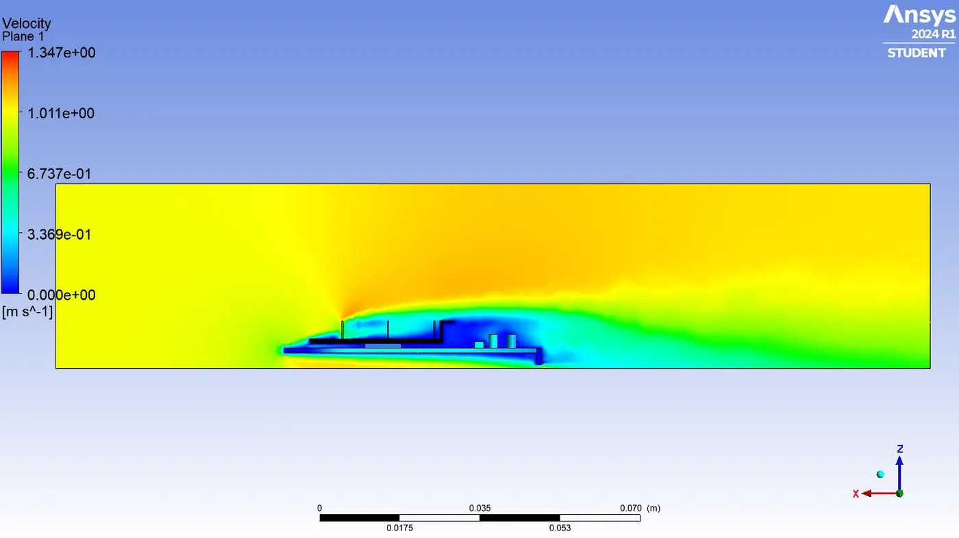
Velocity contour (XZ plane):

velocity vector (XZ Plane):

For copper material in Fins:

• For example, here we are trying to reduce the temperature of fins and processor. so for instance we are using copper material only for fins.

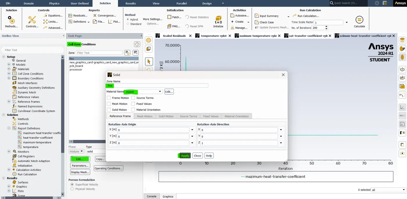
• To set the copper material for fins we need to change the material from aluminum to copper in the cell zone.

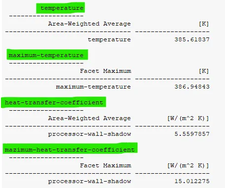
Result:-

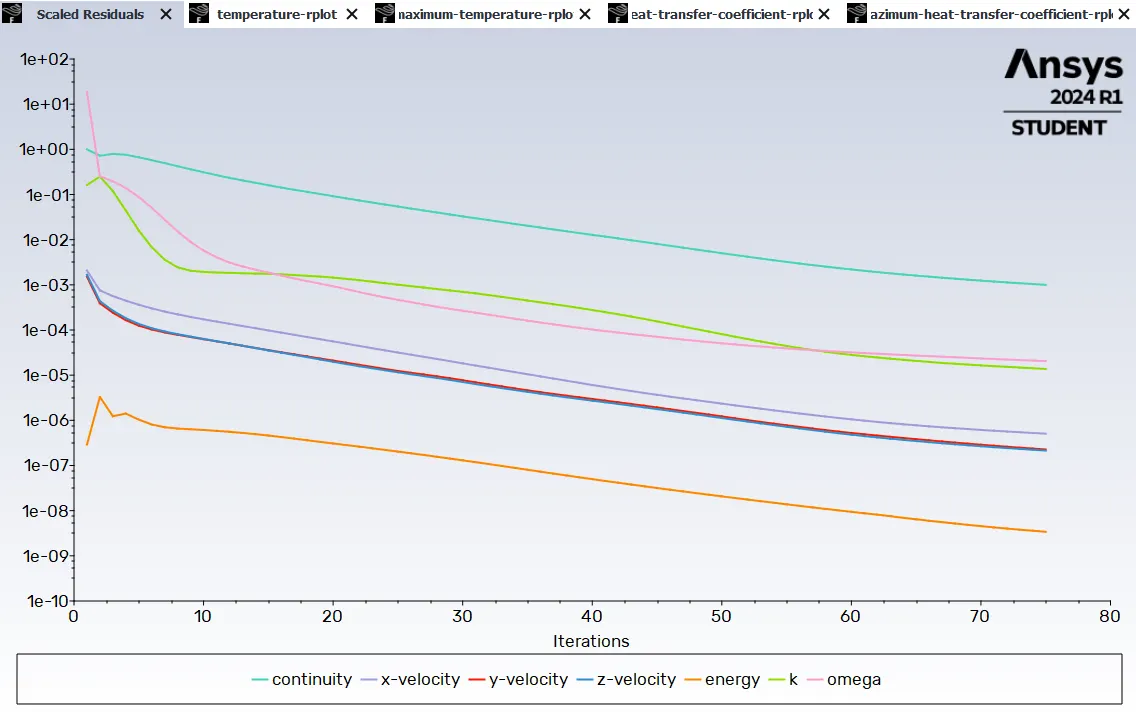
Residuals plot:

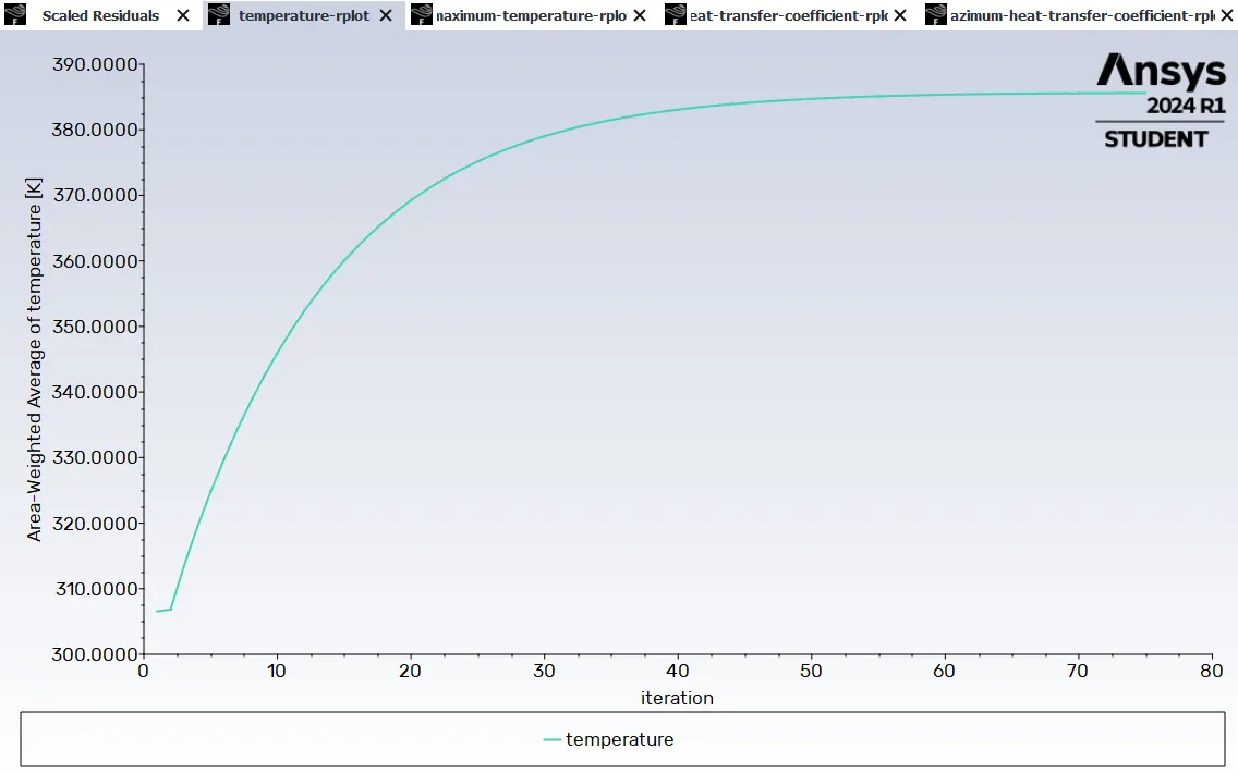
Average Temperature plot (processor):

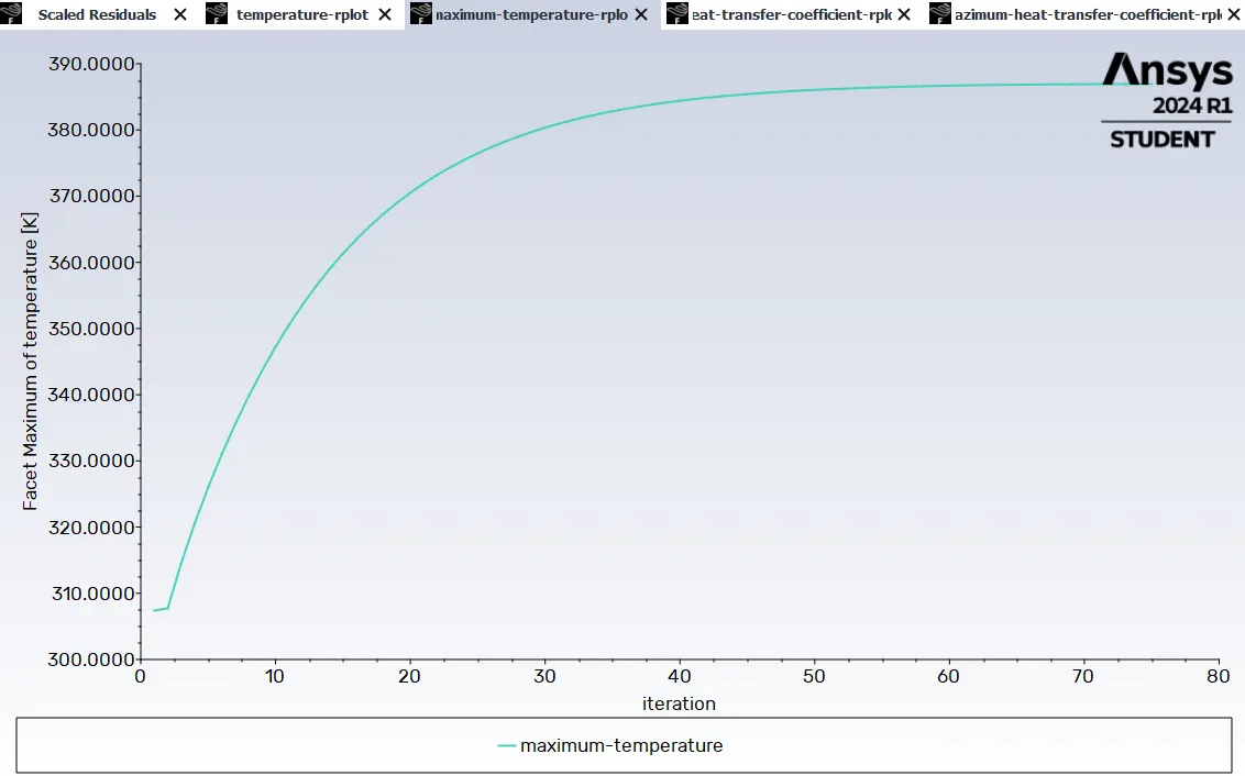
Maximum Temperature Plot (processor):

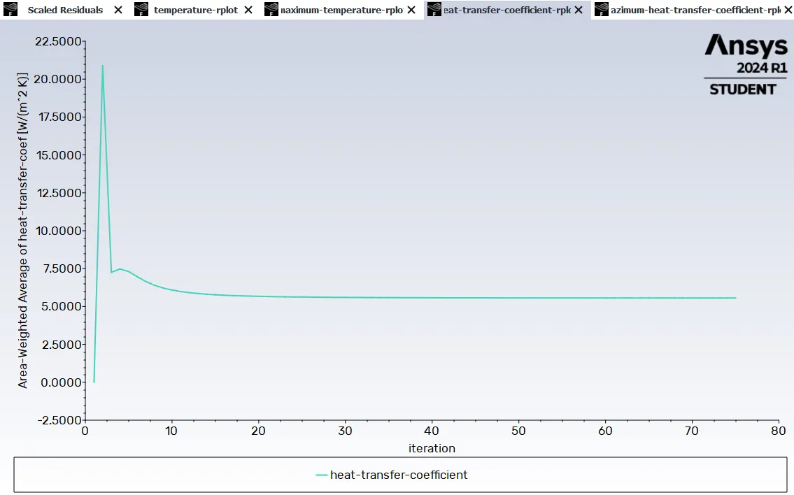
Average Heat transfer coefficient (processor):

Maximum Heat transfer coefficient (processor):

Temperature contour (Processor):-

Heat transfer co-efficient contour (Processor):

Post-processor and solver setting:-

Temperature contour (fins, processor, PCB):

Temperature contour (XZ plane):

Velocity contour (XZ plane):

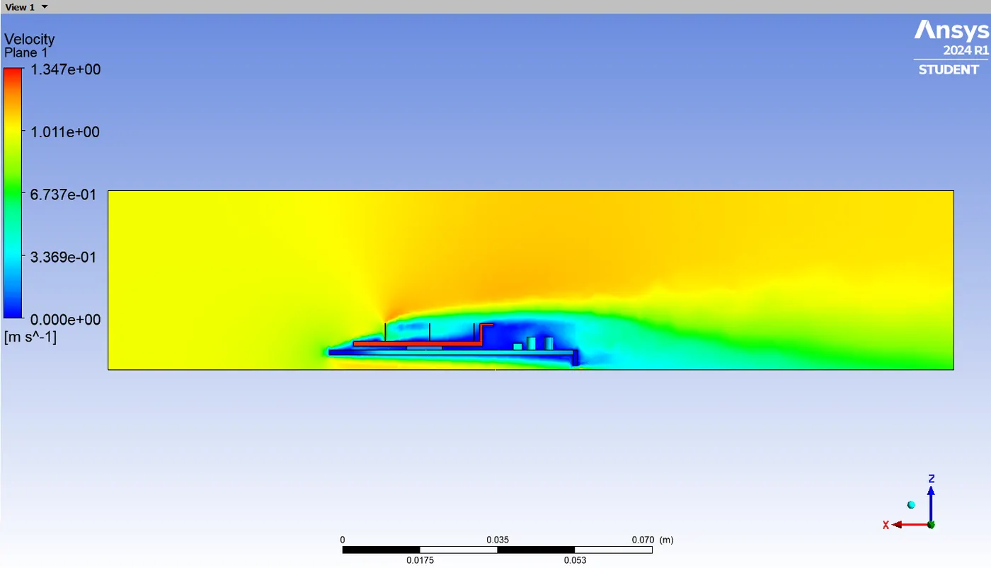
velocity vector (XZ Plane):

Case-3 (Refined mesh, v=3 m/s)

Setup & modeling approach:-

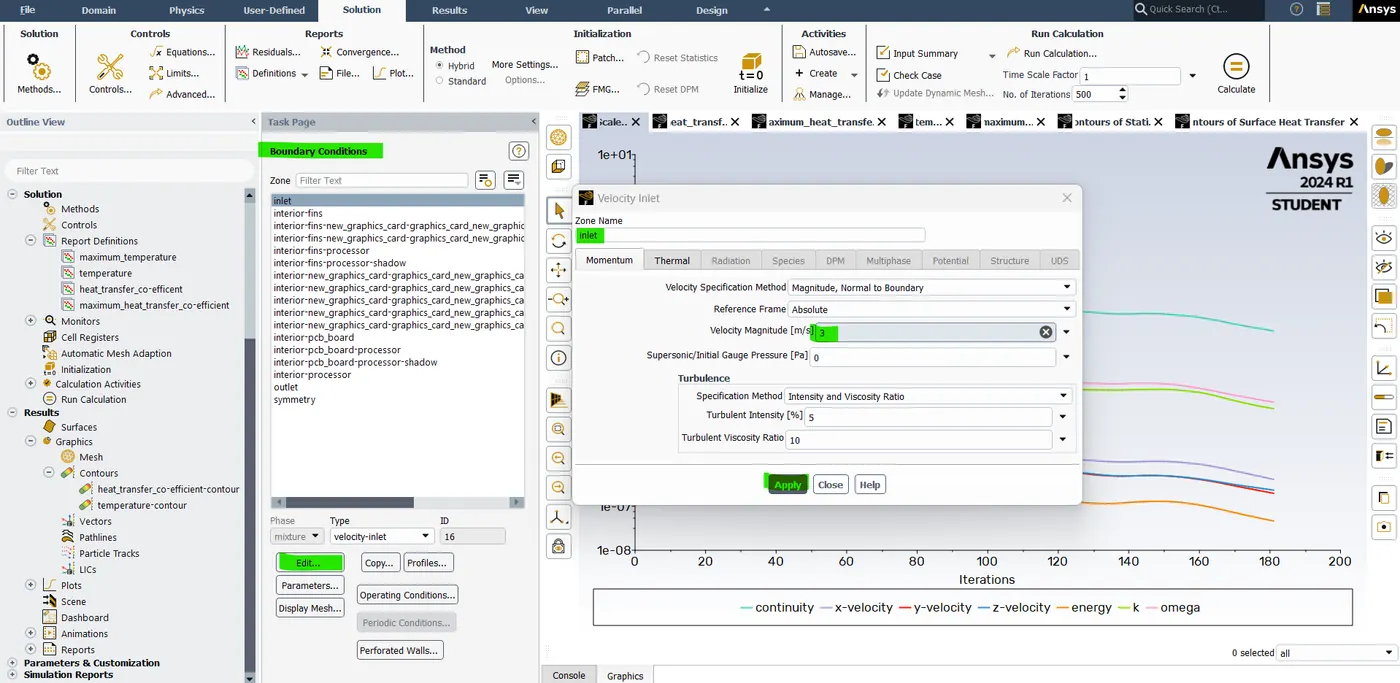
• Follow the same steps which we followed in case 2 for the geomentry and meshing and setup module.
• Here only change in the boundary conditions for the Inlet is 3m/s, the temperature is 300 K and the outlet is 0m/s. And then hit apply.

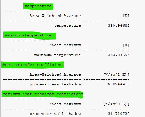
Result:

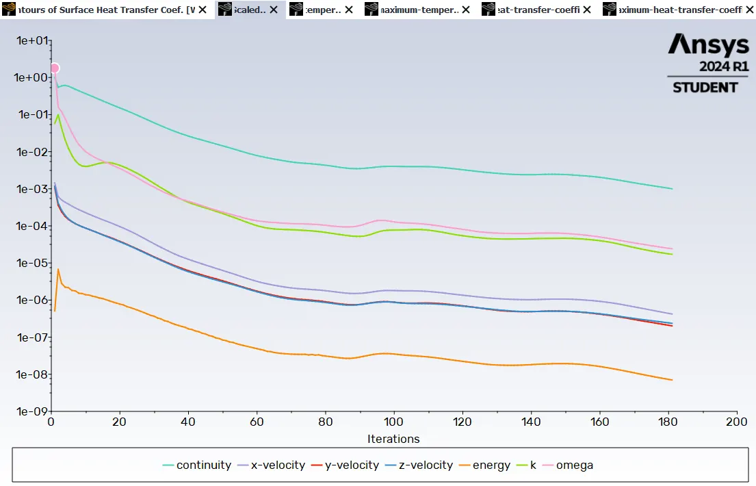
Residuals plot:

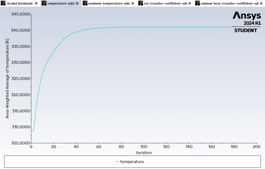
Average Temperature plot (processor):

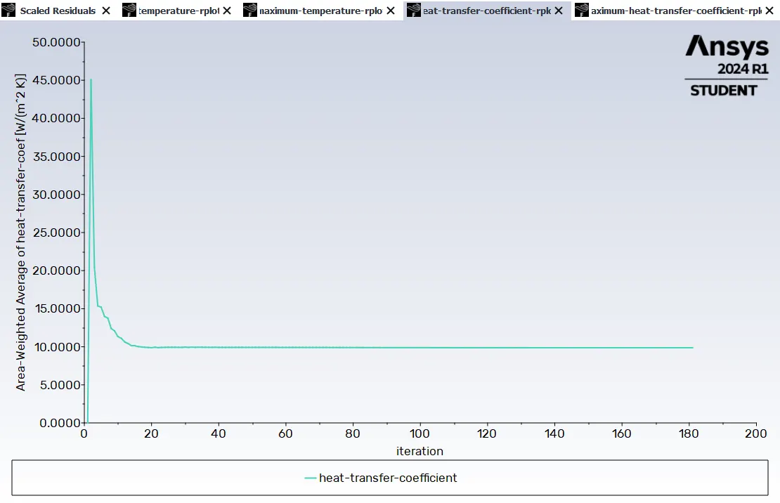
Average Heat transfer coefficient (processor):

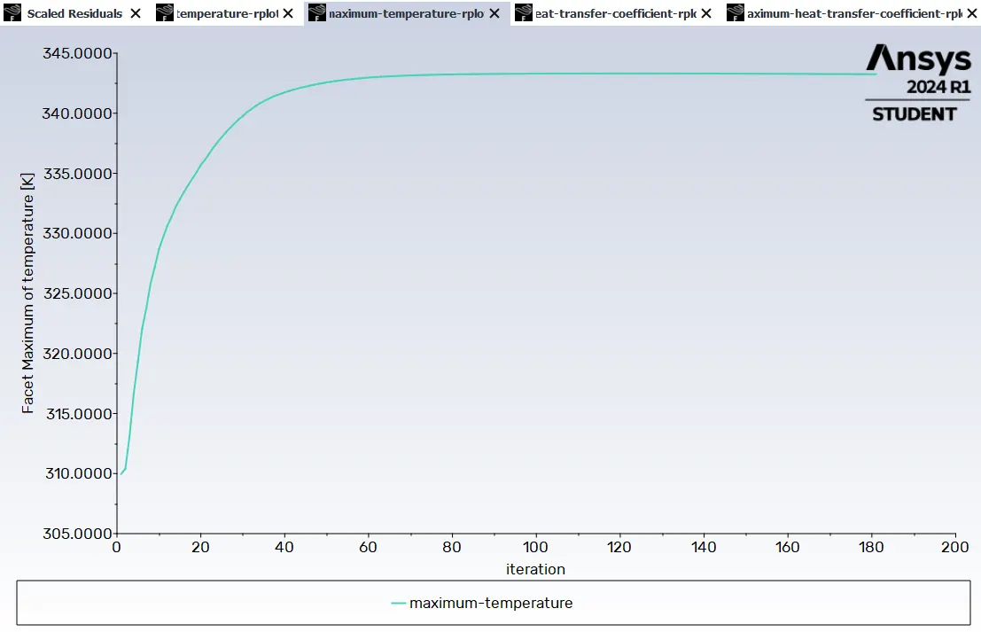
Maximum Temperature Plot (processor):

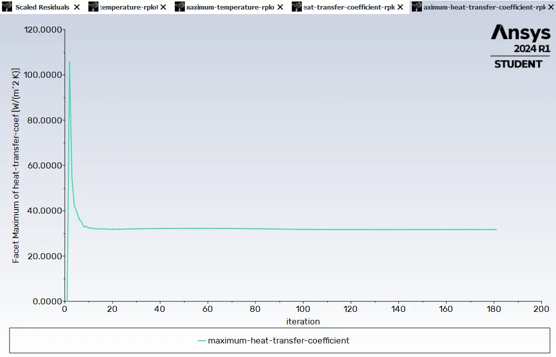
Maximum Heat transfer coefficient (processor):

Post-processing:

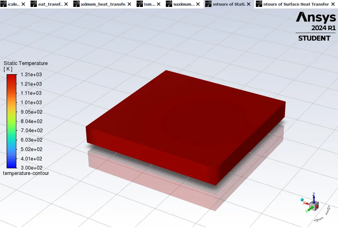
Temperature contour (Processor):

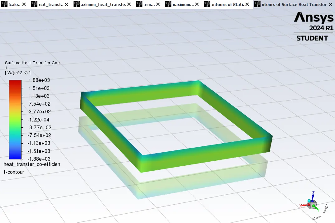
Heat transfer co-efficient contour (Processor):

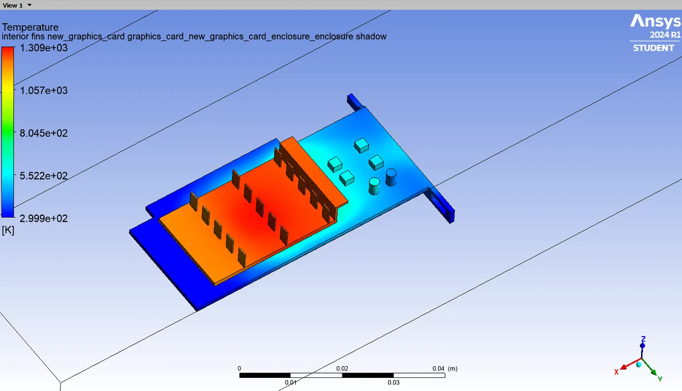
Temperature contour (fins, processor, PCB):

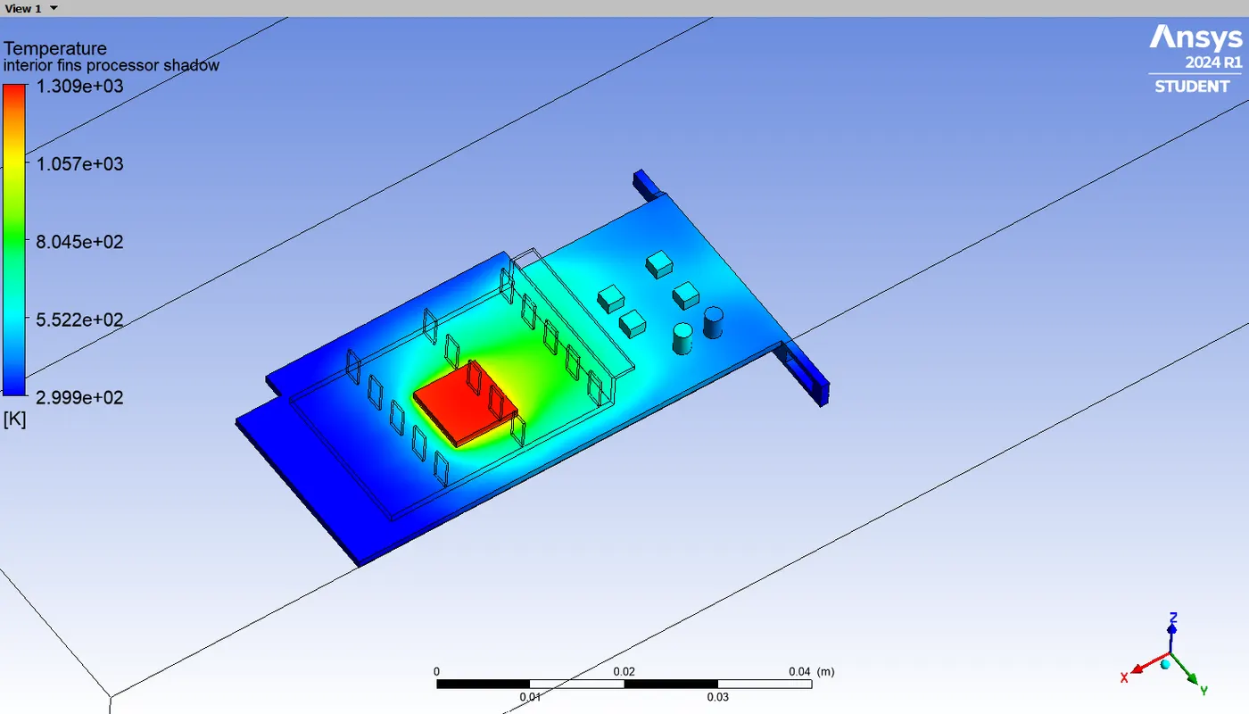
Temperature contour (XZ plane):

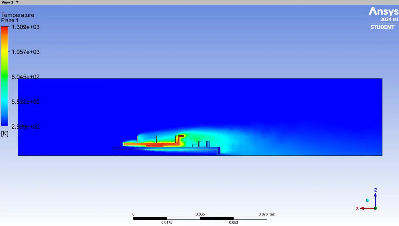
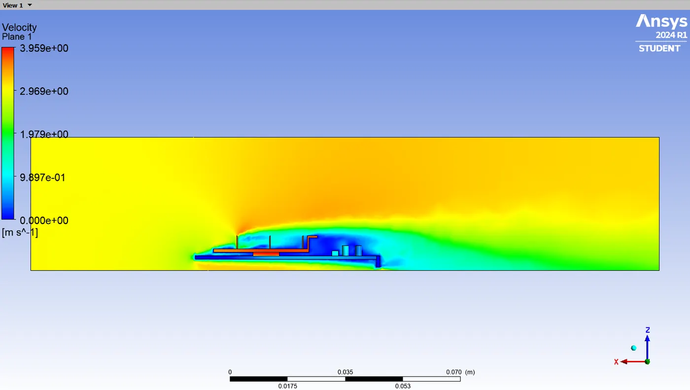
Velocity contour (XZ plane):

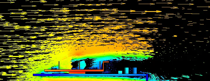
velocity vector (XZ Plane):

For copper material in Fins:-

• For example, here we are trying to reduce the temperature of fins and processor. so for instance we are using copper material only for fins.

• To set the copper material for fins we need to change the material from aluminum to copper in the cell zone.
  

Result:

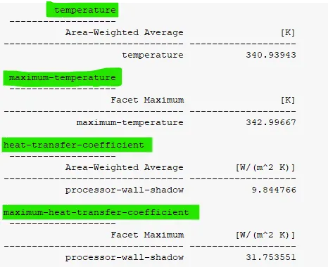
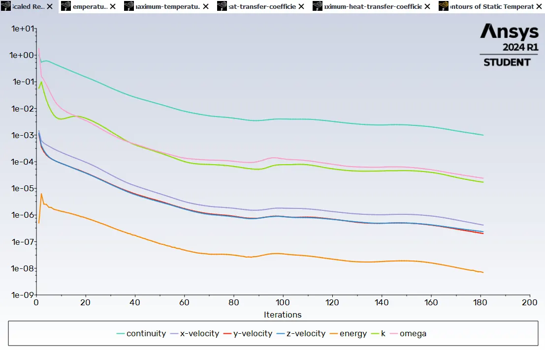
Residuals plot:

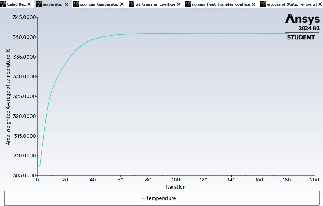
Average Temperature plot (processor):

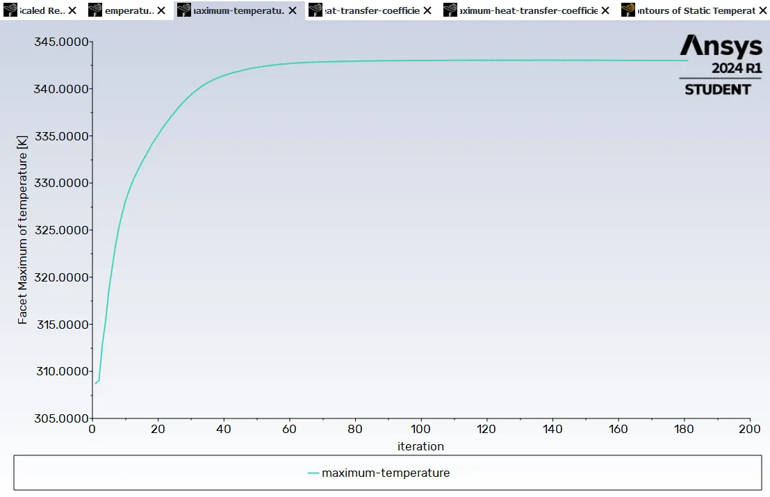
Maximum Temperature Plot (processor):

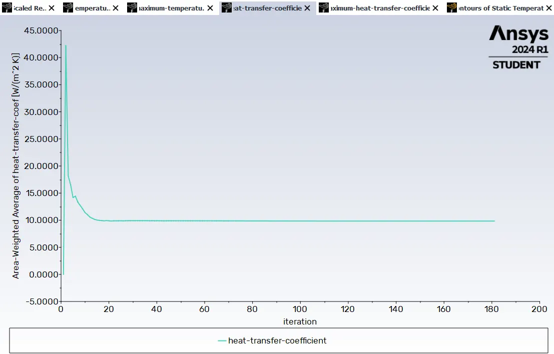
Average Heat transfer coefficient (processor):

Maximum Heat transfer coefficient (processor):

Post processor:

Temperature contour (Processor):

Heat transfer co-efficient contour (Processor):

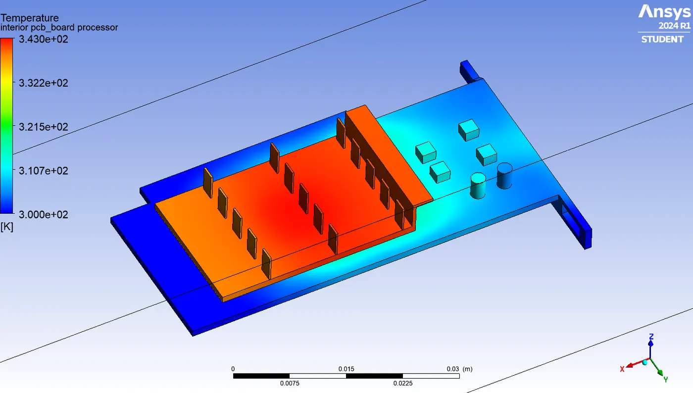
Temperature contour (fins, processor, PCB):

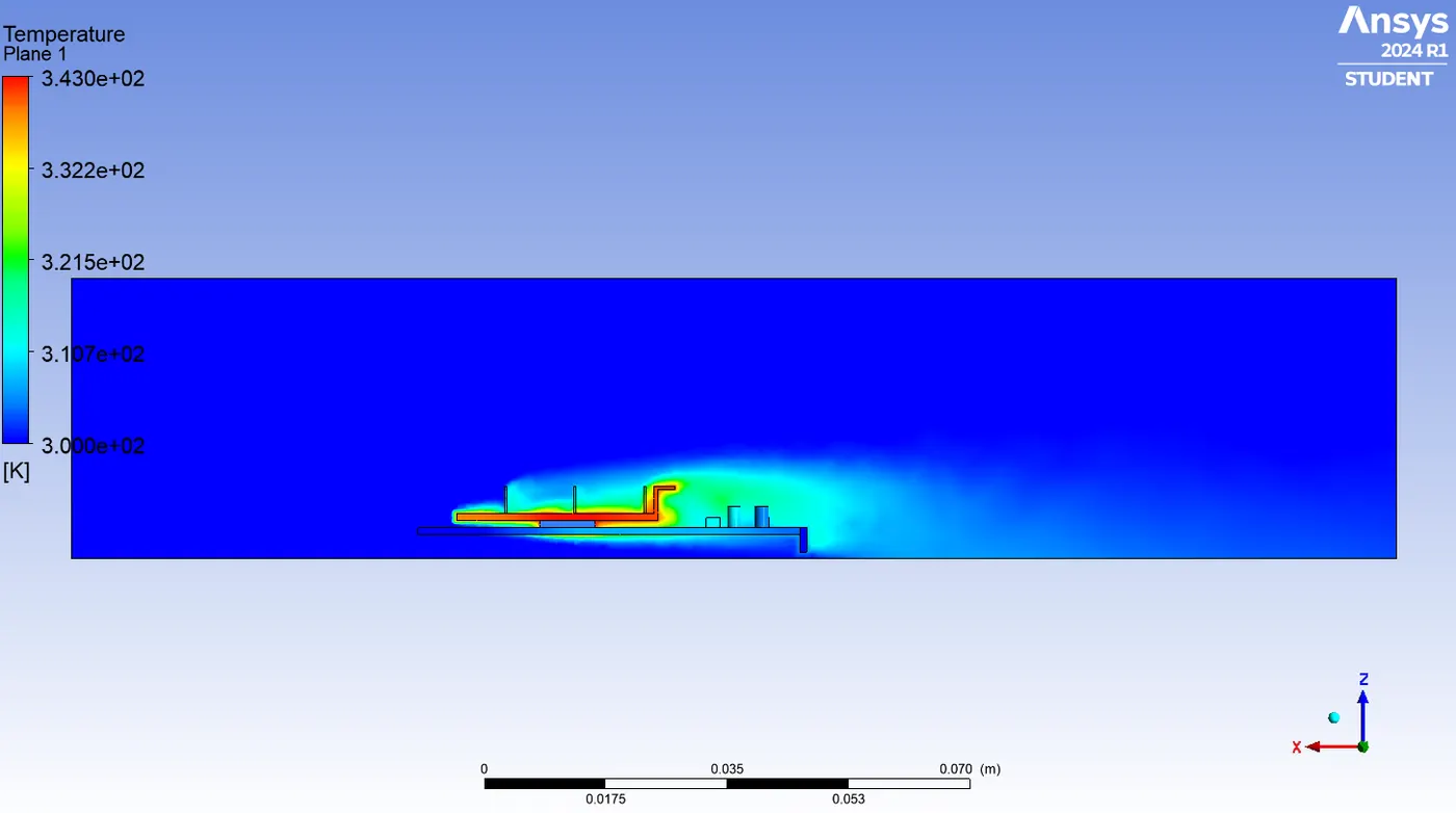
Temperature contour (XZ plane):

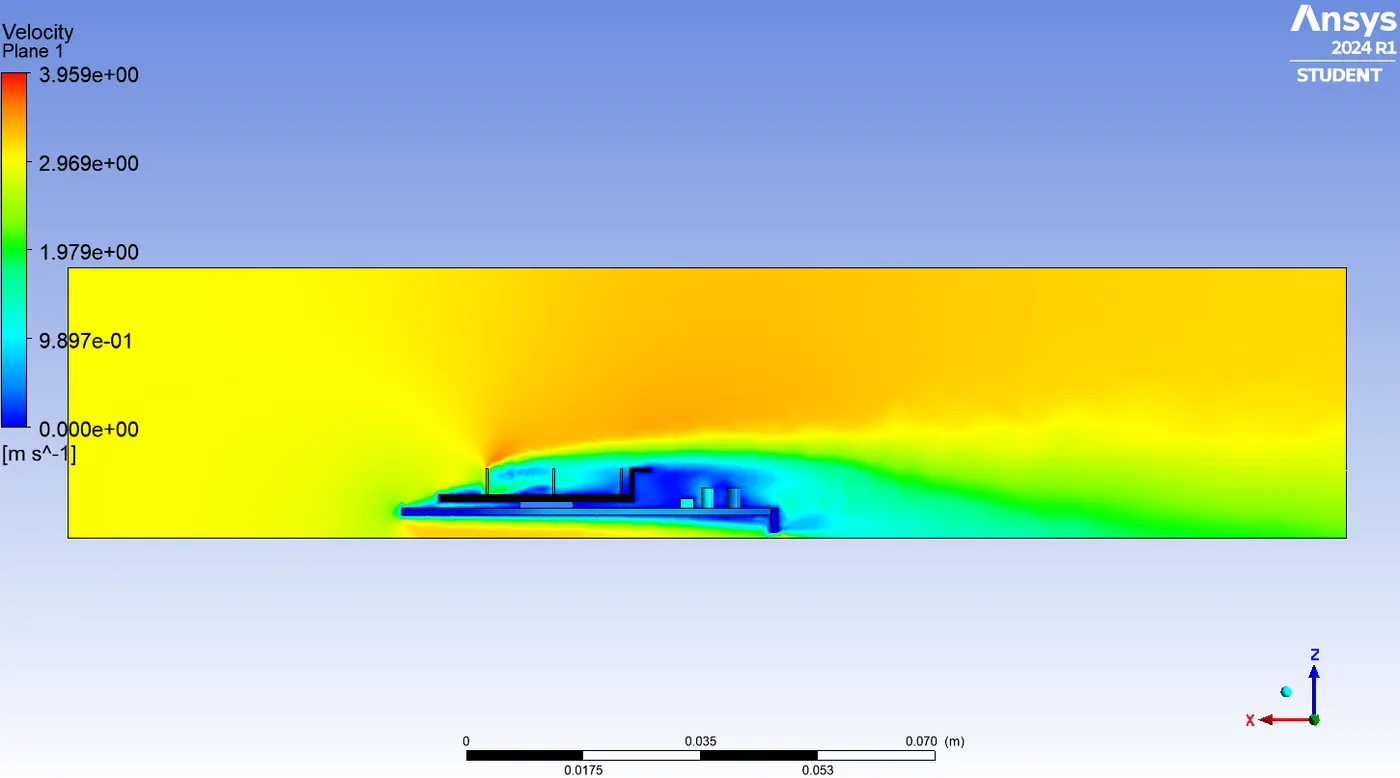
Velocity contour (XZ plane):

Velocity vector (XZ Plane):

Case-4 (Refined mesh, v=5 m/s)

Setup & modeling approach:-

• Follow the same steps which we followed in case 2 for the geomentry and meshing and setup module.
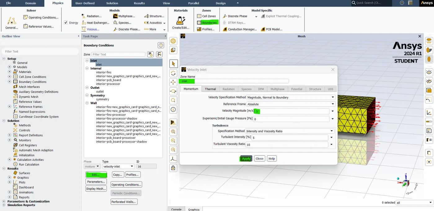
• Here only change in the boundary conditions for the Inlet is 5m/s, the temperature is 300 K and the outlet is 0m/s. And then hit apply.

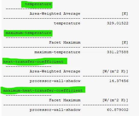
Result:

Residuals plot:

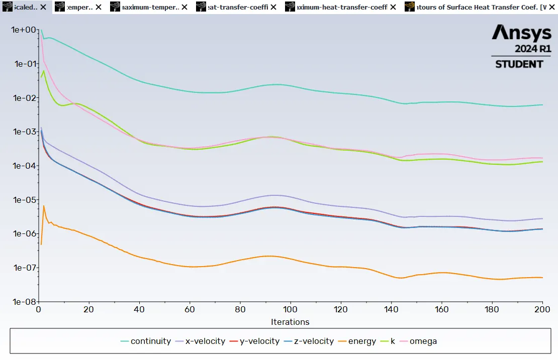
Average Temperature plot (processor):

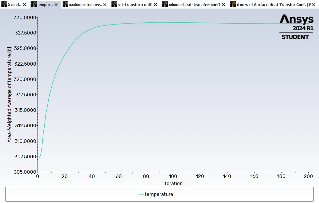
Average Heat transfer coefficient (processor):

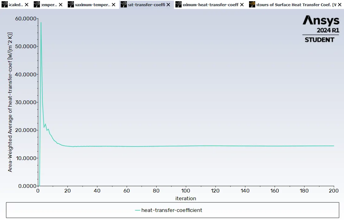
Maximum Temperature Plot (processor):

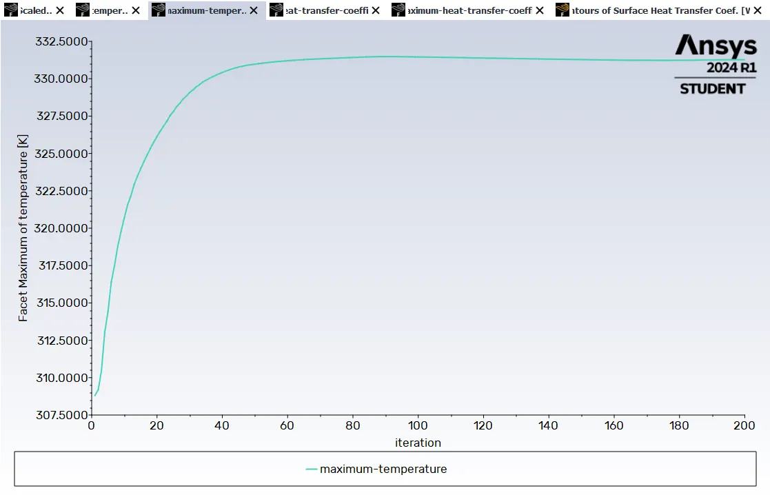
Maximum Heat transfer coefficient (processor):

Post processor:

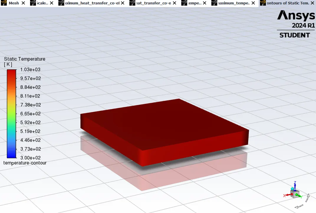
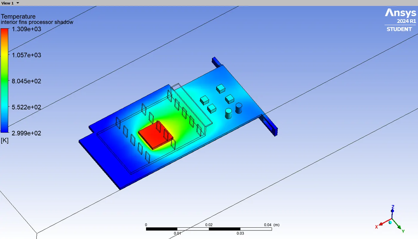
Temperature contour (Processor):

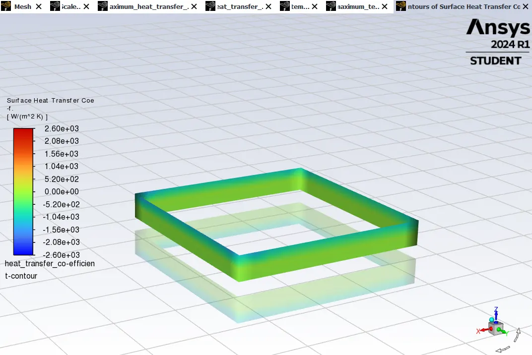
Heat transfer co-efficient contour (Processor):

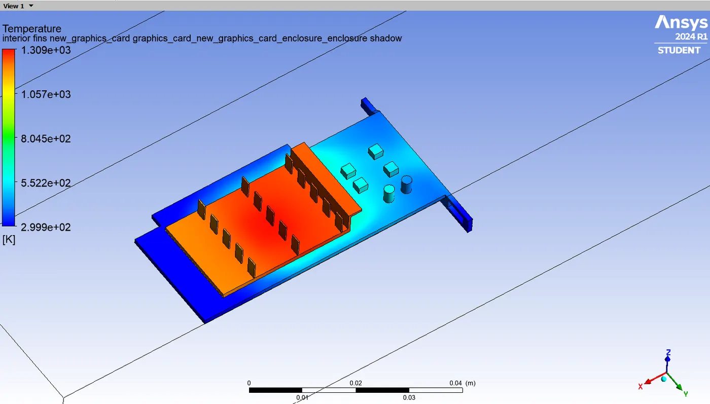
Temperature contour (fins, processor, PCB):

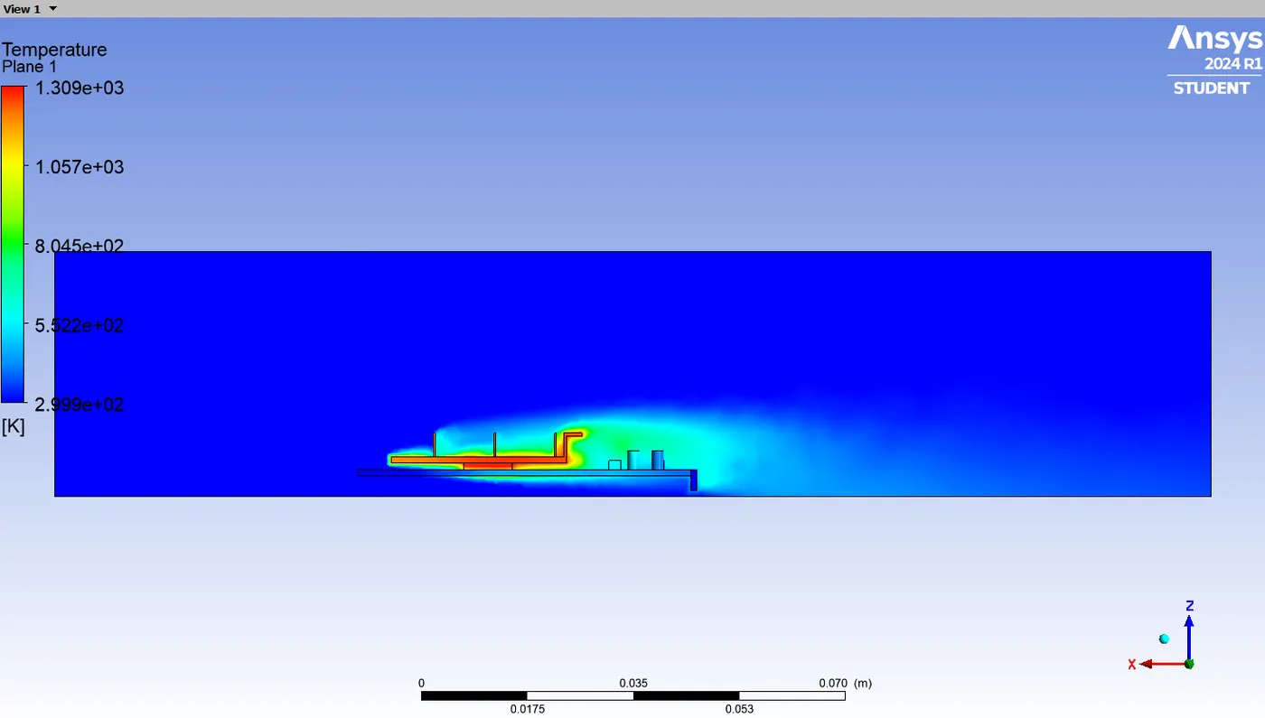
Temperature contour (XZ plane):

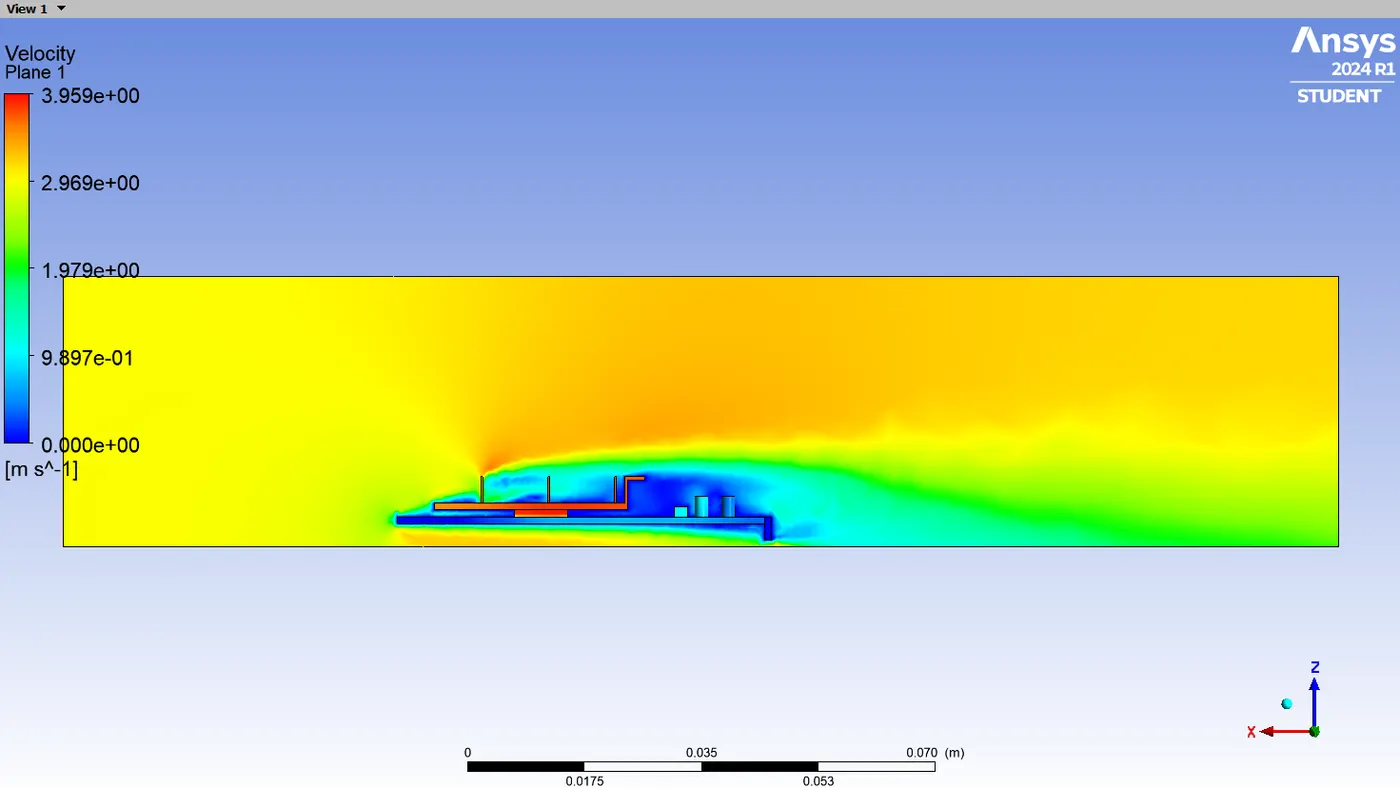
Velocity contour (XZ plane):

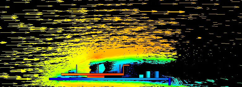
Velocity vector (XZ Plane):

For copper material in Fins:

• For example, here we are trying to reduce the temperature of fins and processor. so for instance we are using copper material only for fins.

• To set the copper material for fins we need to change the material from aluminum to copper in the cell zone.
  

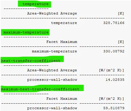
Result:

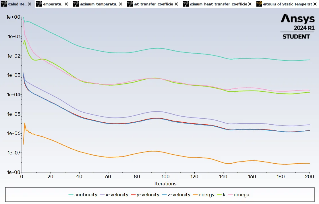
Residuals plot:

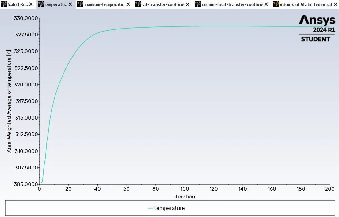
Average Temperature plot (processor):

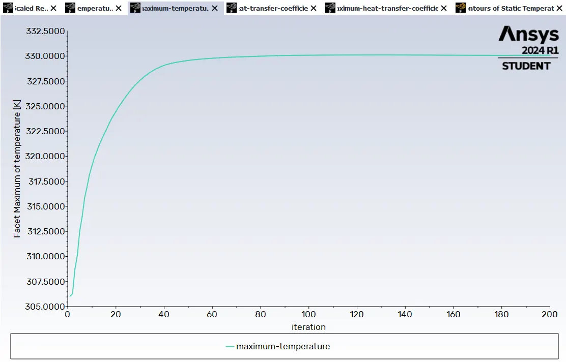
Maximum Temperature Plot (processor):

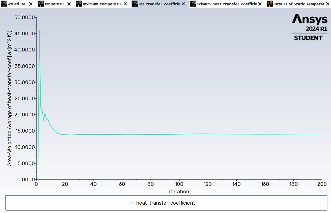
Average Heat transfer coefficient (processor):

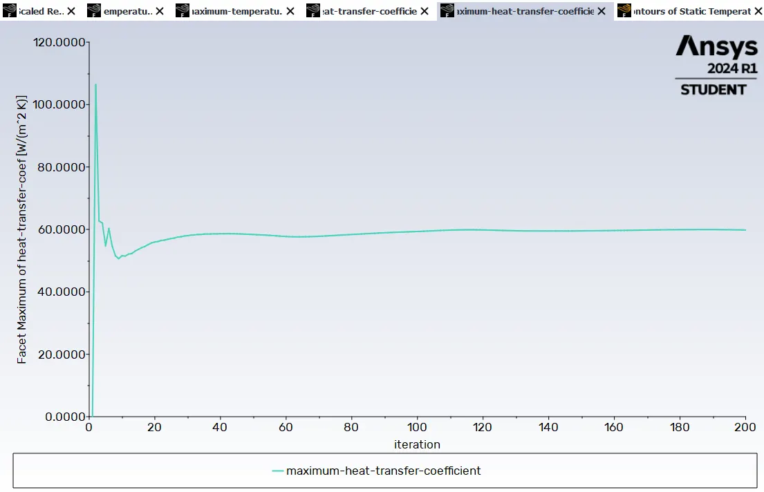
Maximum Heat transfer coefficient (processor):

Post processor:

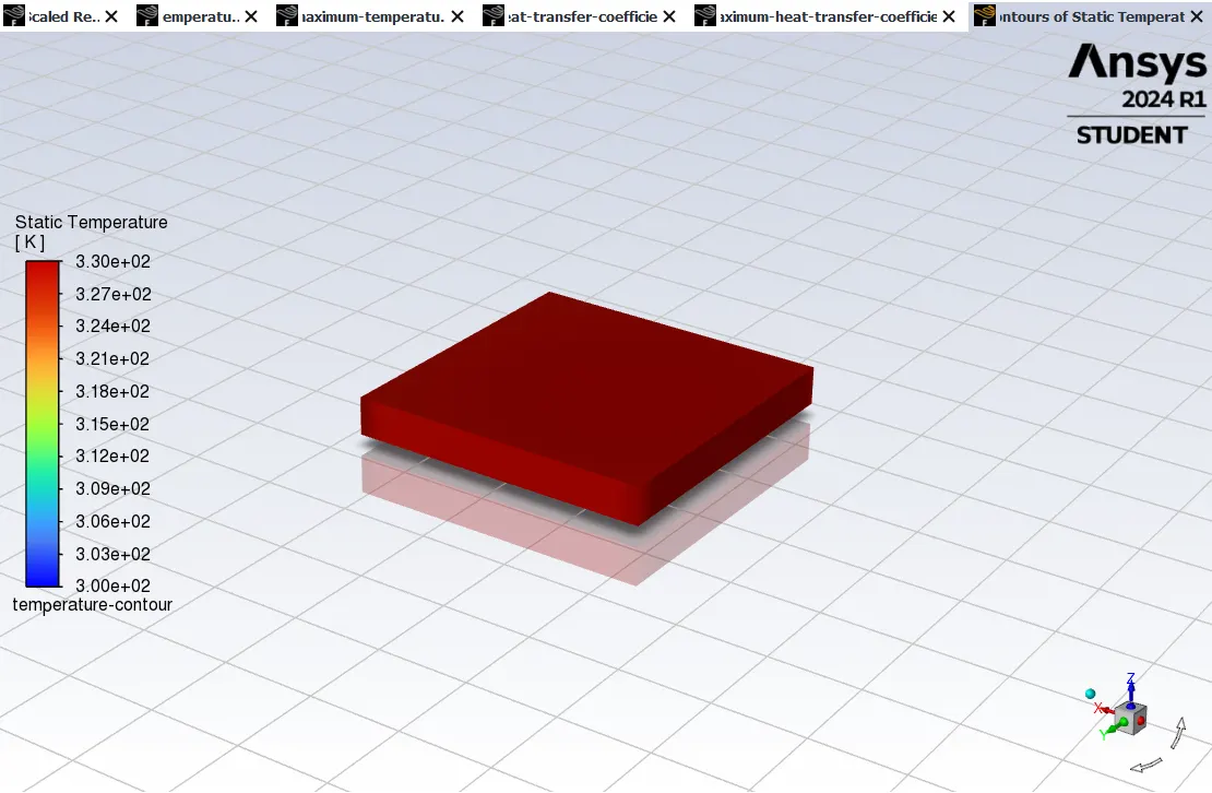
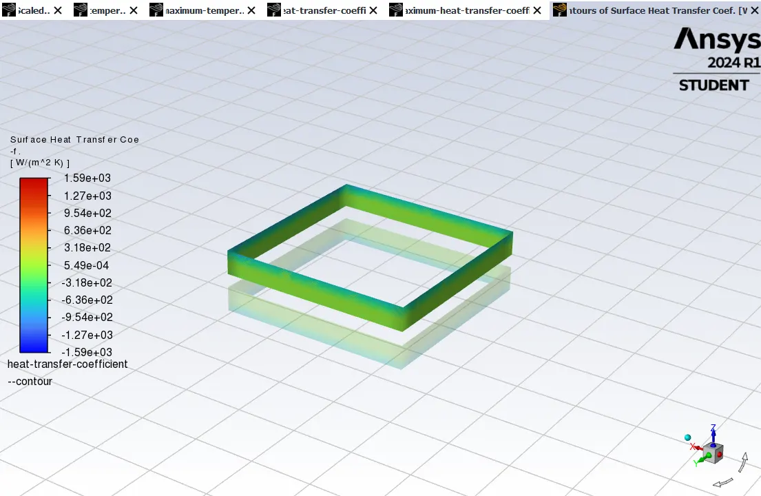
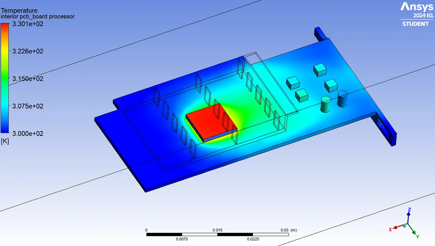
Temperature contour (Processor):

Heat transfer co-efficient contour (Processor):

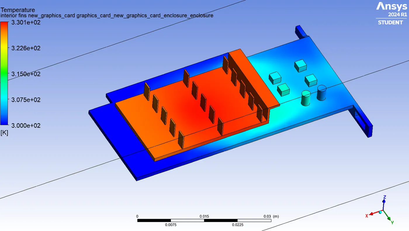
Temperature contour (fins, processor, PCB):

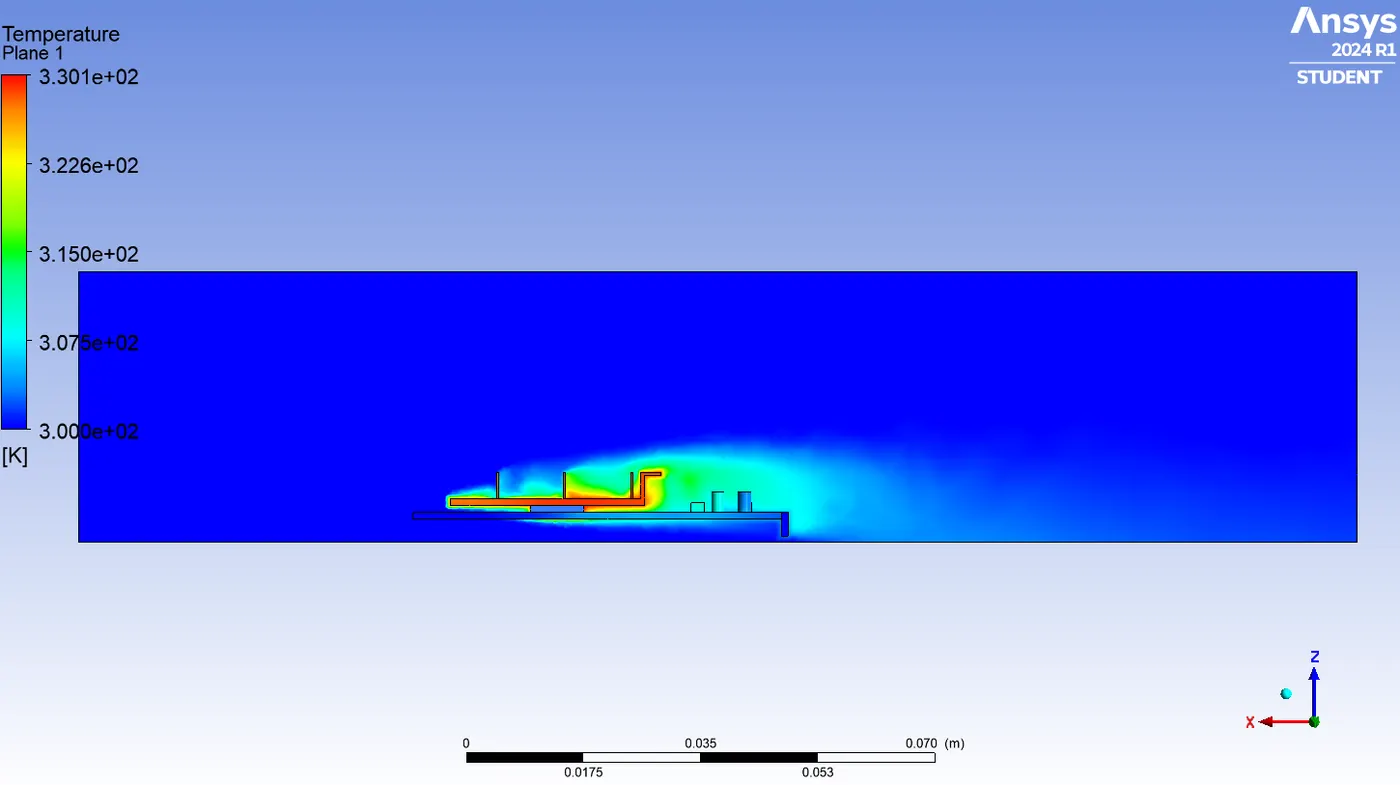
Temperature contour (XZ plane):

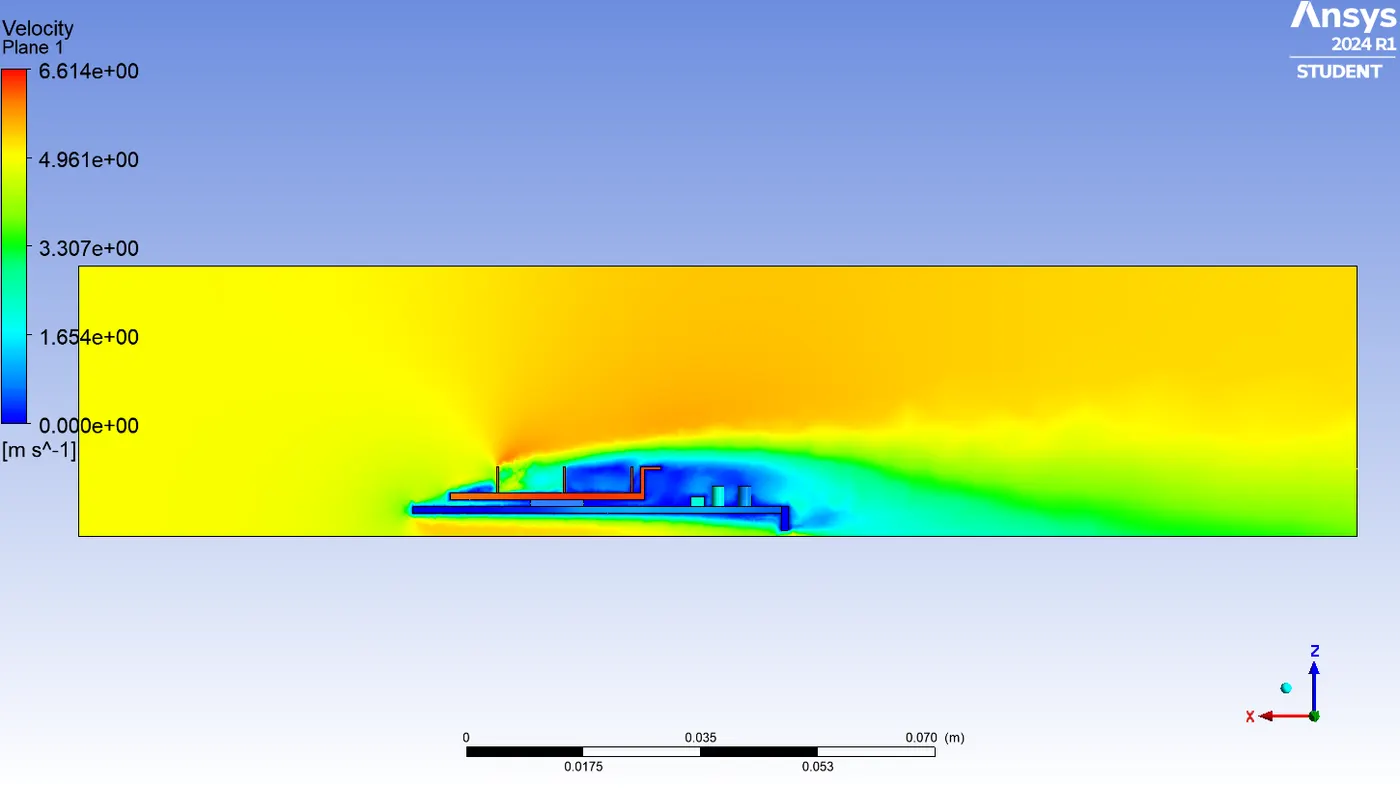
Velocity contour (XZ plane):

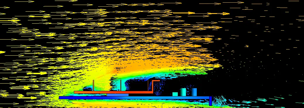
Velocity vector (XZ Plane):

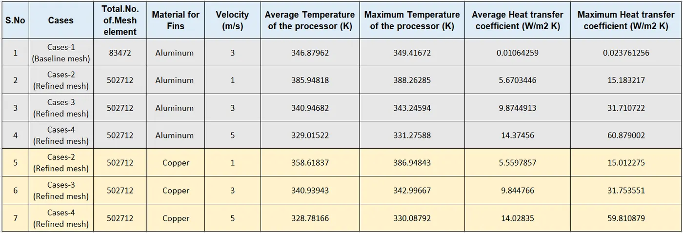
Result:

Conclusion:-

• From the above table, we can observe that if we increase the air's inlet velocity. The convection of the heat transfer coefficient of the air over the processor rises due to which the temperature of the processor decreases.
• Also we can see that for the case with 3 m/s inlet velocity, the baseline mesh, and refined mesh element size vary between the two cases. Since the refind mesh has a higher mesh element size so, it gives more accurate results compared to the baseline mesh. At the same time, the baseline mesh takes less computational baseline, mesh compared to the refined mesh case so, it doesn't provide accurate results.
• In refined mesh, as velocity increases, the heat transfer rate also increases. hence lower the temperature at the surface graphics card but in baseline mesh the values are so random. As the cell count of refined mesh is greater, it has greater accuracy and the computational time is also increased. so, I choose the refined mesh to get the best and most accurate result for this simulation.
• We weren't able to test the grid independence test because we are using this student version of software we've already reached the maximum limit number.of.cells. in this software.

Temperature conture (Fins, PCB, Processor):

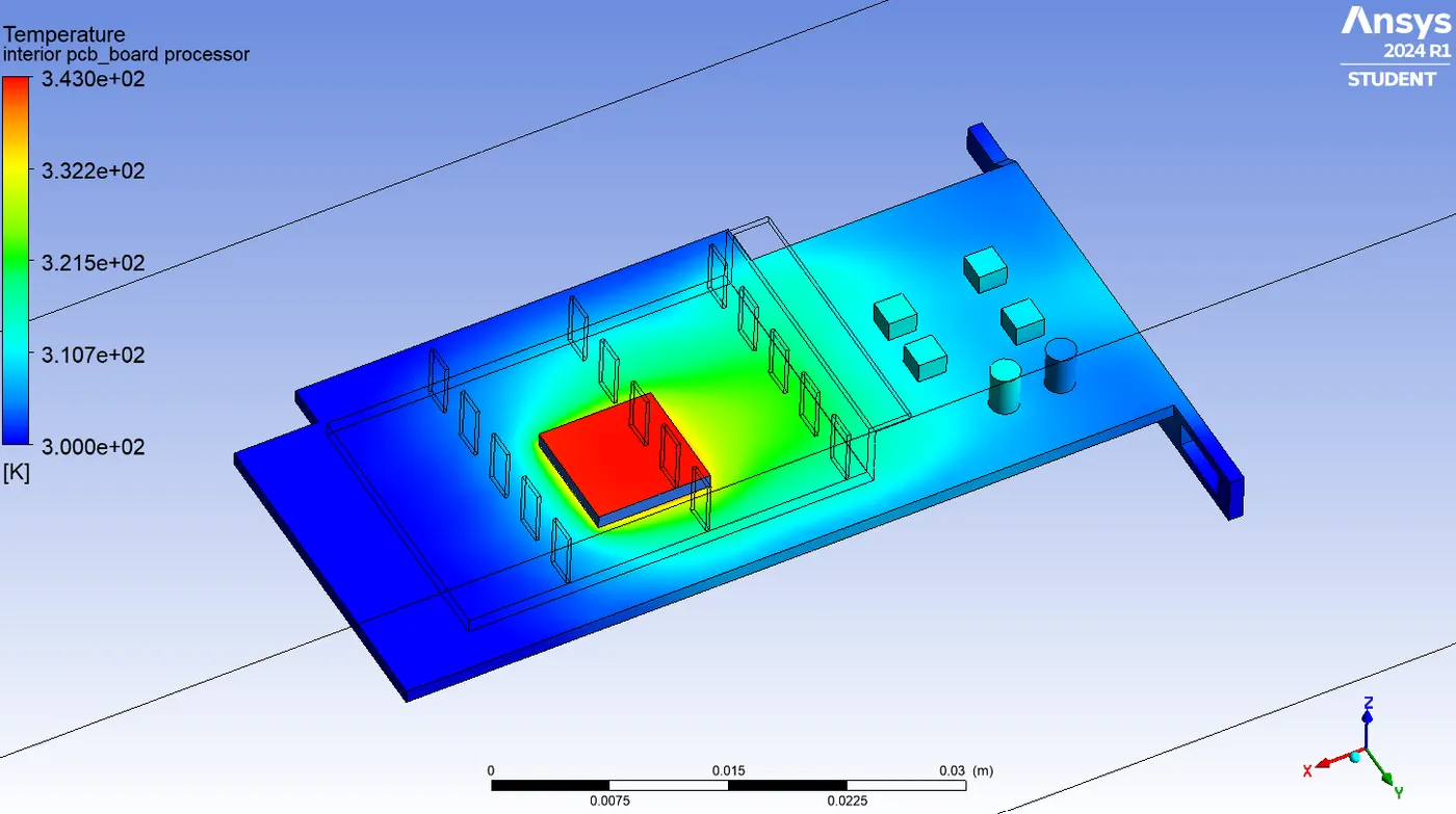
From the above contour, the temperature is maximum at the center portion of the fins region. This is because the processor is the heat source from which the heat is generated and then it is transferred to the surrounding air through convection, and the fins through conduction.

Temperature Conture (Processor):

Heat transfer coefficient contour (Processor):