Week 6 - CHT Analysis on a Graphics card
AIM: To run the simulation for different velocity and to find the respective temperature corresponding to that.
About CHT analysis: It is basically used to calculate the heat transfer coefficent amoung the region of differential heat transfers, eg: conduction through solids, forced convection, etc;
Procedure:
1. Step file imported in ansys space-claim
2. Share topolgy has been done, to get the require conformal mesh
3. after that, mesh has been created, following are the details: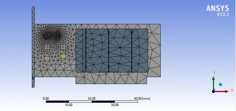
element size: 5mm
Total nodes: 17911
total elements: 81656
and name assignement were also done in this section:
Fins,
Base,
Processor,
Inlet,
Outlet,
Symmetry Wall
4. then, we enter the setup tab, where we choose the pressure based steady based solved, and activating the energy, and choosing the k-epsilon model for analysis,
Material Selection were also done:
Base: Titanium
Fin: Aluminum
Processor: Gold
Boundary Condition were also assigned:
Inlet Velocity: 5 m/s , To=300K
Also giving a 9e7 w/m^3 as a thermal energy generation to processor
5. Following Results were obtained:
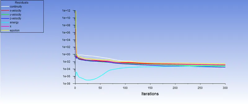 Fig: Residual Plot, indicating the convergence of solution
Following are the static temperature plot:
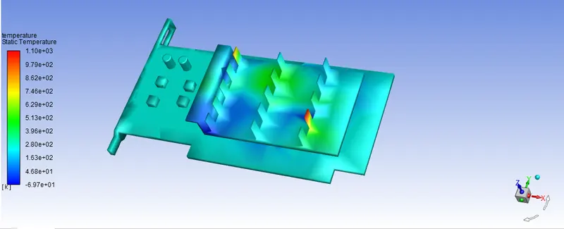
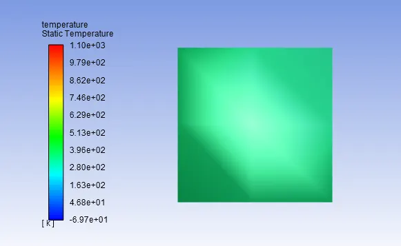
Fig: Processor Temperatuer Profile (500 k)
Refined Mesh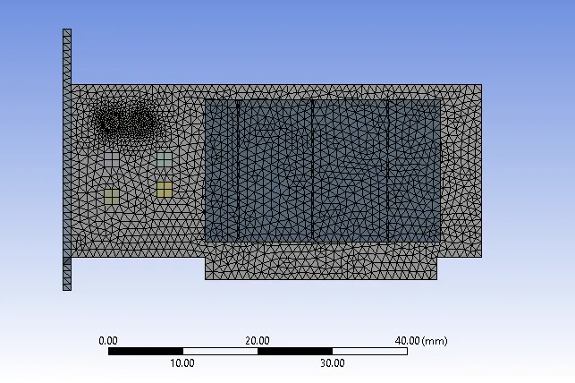
Element Size: 1mm
Total Element: 270205
Total Nodes: 1424900
Following are the post processsing results for the 5m/s veloity:
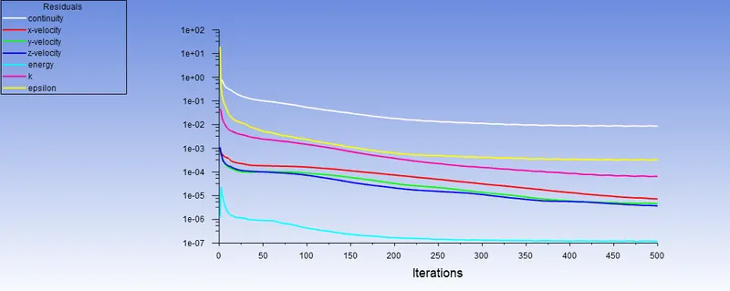 Fig: Residual Images, showing convergnece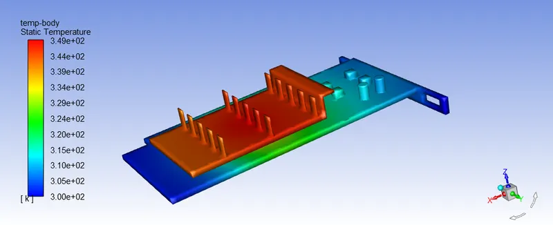
Fig: Indicating Temp Contour
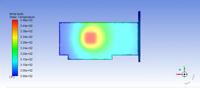 Fig: Indicatingtemp contour back side
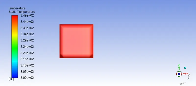 Fig:indicating temp contour of processor (350 K)
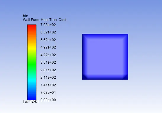
Fig: indicating HTC of processor (70qq3)
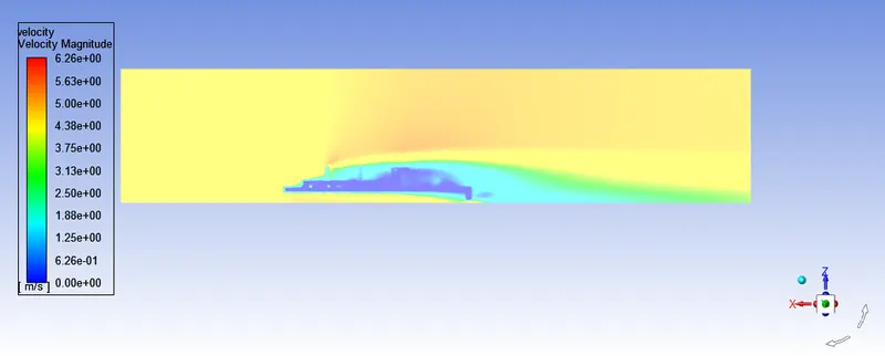 Fig: indicating Velocity contour
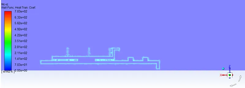 Fig: indicating HTC contour on plane
FOllowing are the simulation images for 3m/s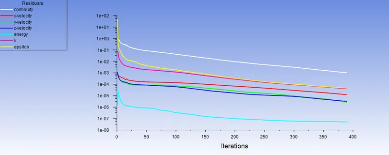
Fig: indicating the residual, (convergence)
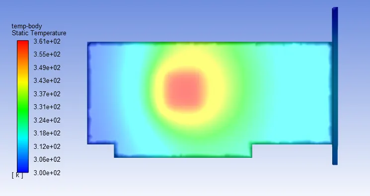 Fig: indicating the temp contour (bottom side)
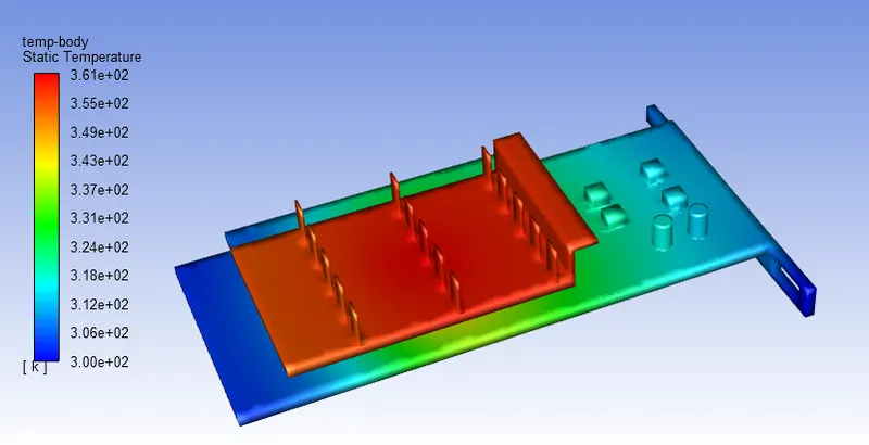 Fig: indicating the temp contour
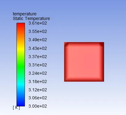
Fig: indicating the temp contour for processor
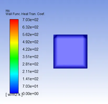
Fig: indicating the HTC for processor
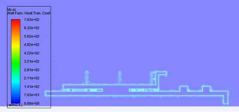 Fig: indicating the HTC
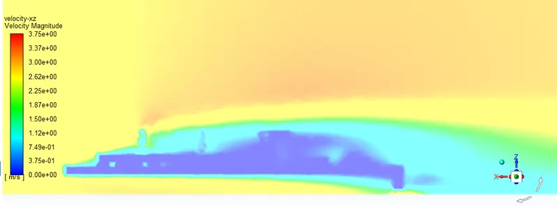 Fig: indicating the velocity flow over plane
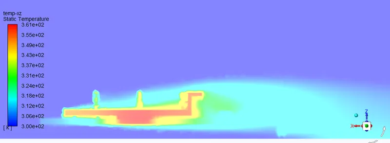 Fig: indicating the temp flow over the plane
Following are the result for the 1m/s
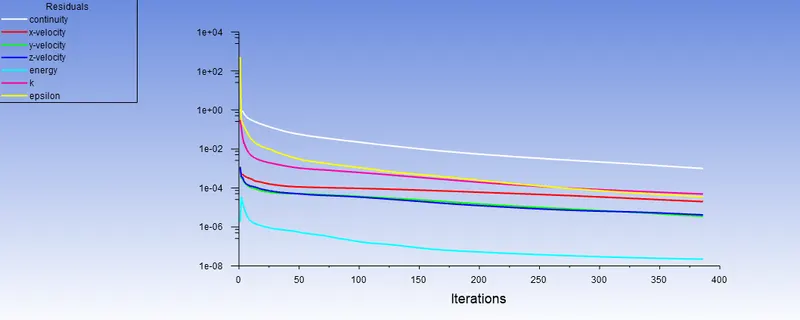 Fig: Indicating the Convergence
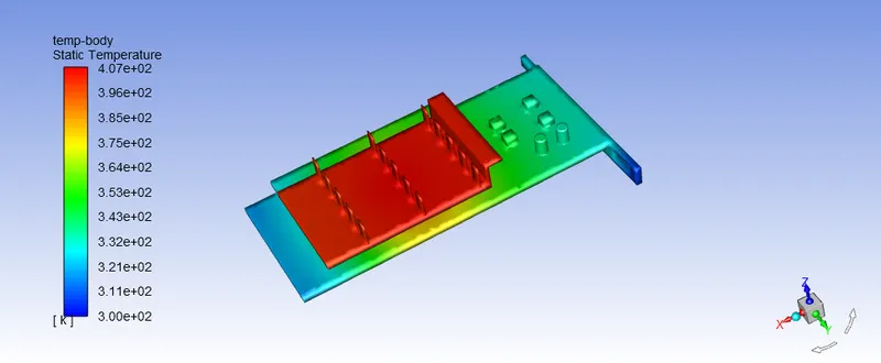 Fig: Indicating the temp contour
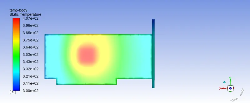 Fig: indicating the temp contour for bottom of body
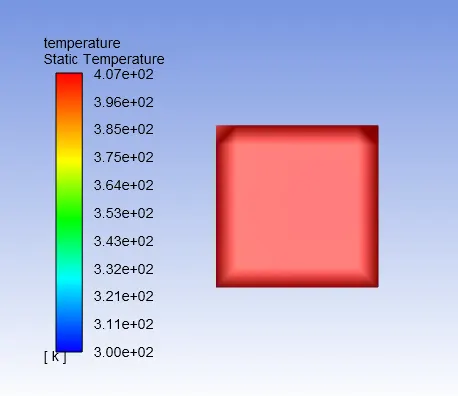
Fig: temp contour for processor
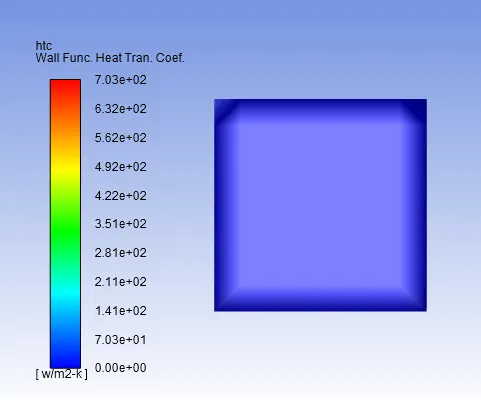
Fig: htc contour for processor
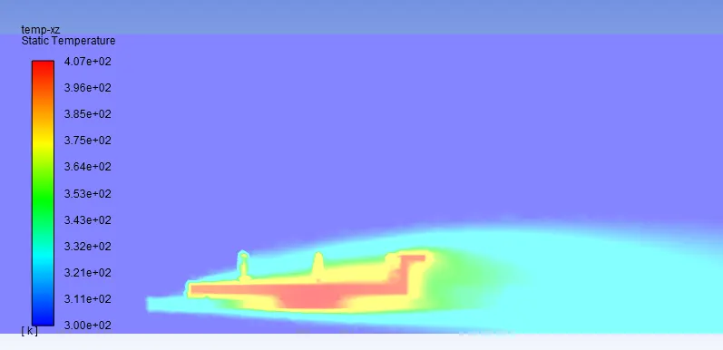 Fig: indicatig the temp on a plane
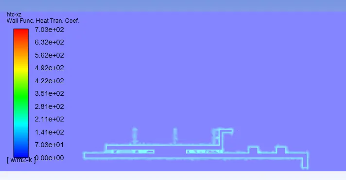
Fig: Indicating the HTC on plane
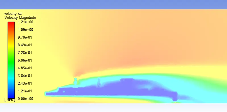 Fig: indicating the velocity on a plane
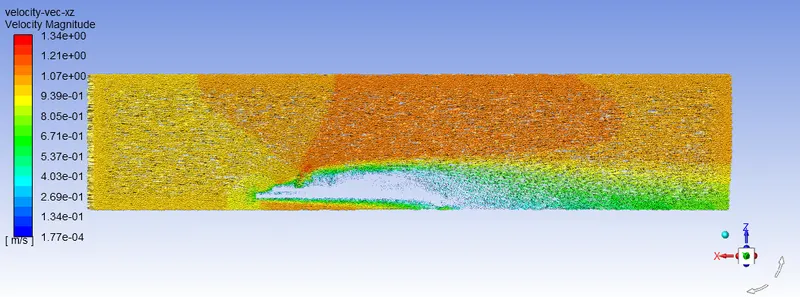 Fig: indicating the velocity on a plane over the surface
Following are the comparitive analysis for the above three velocities:
| Processor Stats | ||
| Velocity (m/s) | Max Temperature (K) | HTC (W/m^3) |
| 5 | 349 | 703 |
| 3 | 361 | 703 |
| 1 | 407 |
703 |
1. it is observed that, as the velocity increases, the temperature decreases, which suggest, at higher velocity the cooling efficiency is greater as compared to earlier version.
2. the value of HTC is kept constant over the whole range of velocity, as the value of HTC is not depend upon the velocity.
3. as the element size decreases, the more refine the mesh, the better the result we get.