Week 6 - CHT Analysis on a Graphics card
Aim:
Perform a steady-state conjugate heat transfer analysis on a model of a graphics card.
Objectives:
Simulate CHT analysis on a graphics card model and use appropriate materials of your choice for the simulation.
Simulate by varying the velocity from 1m/sec to 5m/sec for at least 3 velocities.
Find out the max temperature and heat transfer coefficient attained by the processor.
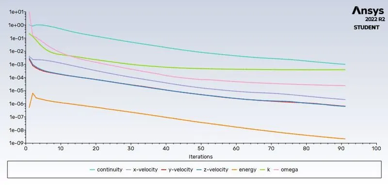
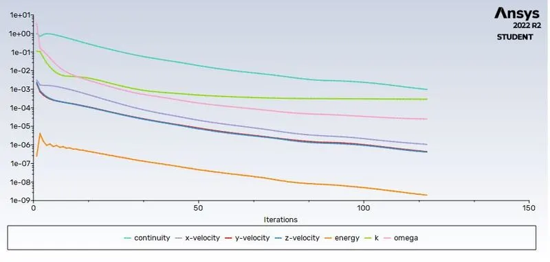
Prove that the simulation has achieved convergence with appropriate images and plots.
Theory:
Conjugate heat transfer:
Conjugate Heat Transfer analysis is used for processes that involve a variety of temperatures concerning solids and fluids, due to thermal interaction between them. A typical example would be the heating or cooling of a solid by the flow of air.
The exchange of heat between two bodies is known as heat transfer and the rate of heat transfer is directly proportional to the temperature difference between them. Heat transfer in solids is usually occurred by conduction whereas in the case of fluids heat transfer occurs by convection. Efficiently combining heat transfers between solids and fluids is the key to designing effective coolers, heaters, or heat exchangers. Forced convection is the most common way to achieve higher heat transfers. For some applications, the performance is further improved by combining convection with phase change(for example liquid water to vapor phase change).
Heat transfers in solids and heat transfers in fluids are usually combined in the majority of applications. This is because fluid flows around solids or between solid walls and usually solids are immersed in the fluids.
An accurate description of parameters such as material properties, flow regimes, geometry configurations, selecting correct models based on the physics to be captured, and heat transfer modes near the boundaries is needed for the analysis of temperature fields and heat transfer.
The Conjugate Heat Transfer (CHT) analysis type allows for the simulation of heat transfer between solid and fluid domains by exchanging thermal energy at the interfaces between them. Typical applications of this analysis type exist as, but are not limited to, the simulation of heat exchangers, cooling of electronic equipment, and general-purpose cooling and heating systems.
Examples
HVAC, Heat Exchanger, Tank, Internal Combustion Engine, Heat Sink, Boiler, Reactor, Heat Pipe, Turbocharger.
Heat Transfer in a Solid - Conduction: Diffusion of heat due to temperature gradients in solids. A measure of the amount of conduction for a given gradient is heat conductivity. Conduction is described by Fourier’s law defining the conductive heat flux, q, proportional to the temperature gradient
Heat Transfer in a Fluid - Convection: When heat is carried away by moving fluid. The flow can either be caused by external influences, forced convection, or by buoyancy forces, natural convection.
Due to the fluid motion, there are three contributions to the heat transfer:
1. Convective contribution: Depending on the properties of the fluid and its region of flow, the domination of conduction and convection varies.
2. Viscous effects: Due to the fluid flow, the viscosity creates heat. This effect is often neglected due to its negligible value but should be taken into account for high-velocity cases.
3. Density effects: When the density relates to the temperature, the domain will have different densities at different locations based on the temperature distribution. This variation in density can cause compression which in turn generates heat.
The contemporary conjugate convective heat transfer model was developed after computers came into wide use to substitute the empirical relation of proportionality of heat flux to temperature difference with the heat transfer coefficient which was the only tool in theoretical heat convection since the times of Newton. This model, based on a strictly mathematically stated problem, describes the heat transfer between a body and a fluid flowing over or inside it as a result of the interaction of two objects. The physical processes and solutions of the governing equations are considered separately for each object in two subdomains. Matching conditions for these solutions at the interface provide the distributions of temperature and heat flux along the body–flow interface, eliminating the need for a heat transfer coefficient. Moreover, it may be calculated using these data.
Applications:
Starting from simple examples in the 1960s, the conjugate heat transfer methods have become a more powerful tool for modelling and investigating natural phenomena and engineering systems in different areas ranging from aerospace and nuclear reactors to thermal goods treatment and food processing, from complex procedures in medicine to atmosphere/ocean thermal interaction in meteorology, and from relatively simple units to multistage, nonlinear processes. A detailed review of more than 100 examples of conjugate modeling selected from a list of 200 early and modern publications shows that conjugate methods are now used extensively in a wide range of applications. That also is confirmed by numerous results published after this book's appearance (2009) that one may see, for example, at the Web of Science. The applications in specific areas of conjugate heat transfer at periodic boundary conditions and in exchanger ducts are considered in two recent books.
Practical CHT problems are used to determine:
The maximum and minimum temperature in various parts of the system. eg: combustion chambers, gas turbines, chemical vessels, etc.
Temperature Distribution is related to the thermal stress over a particular wall or system etc.
Temperature Response in time-dependent applications such as heating/cooling problems (For example, In the case of cooling a particular system such as engine cooling)
Overall heat transfer is co-efficient.
Introduction:
A CHT (Conjugate Heat Transfer) analysis is useful where there are multiple modes of heat transfer in our computational domain, like conduction and convection. Having such a great number of applications for this type of simulation makes it important to be studied in depth.
Assumptions:
1) The air flow profile from the inlet is considered to be of uniform value, instead of a profile of different values.
2) Air flow resistance due to the cabinet's back mesh is considered to be 0.
3) The heat-producing chip is small in size compared to real-life graphic cards, so the heat generation capacity is reduced accordingly.
4) The physical constraints to the flow due to side walls are considered to be zero. (The temperature gradient alongside walls is found to be negligible, so they are replaced with symmetry boundary conditions)
Simulation:
This project is divided into 2 parts based on the Mesh (with a baseline and a refined mesh). The geometries in both parts of the project are the same.
In Part 1, we run 3 different simulations with 3 different mesh sizes (default, medium, and refined mesh size)
In Part 2, we run 3 different simulations with 3 different velocities of 1 m/s, 2.5 m/s, and 5 m/s (using refined mesh).
Part 1:
Geometry setup:
Use Spaceclaim to edit the geometry of the downloaded model of the graphics card which is in the enclosure.
Click on share prep to view any edges in interference so that conformal mesh can be achieved between different components.
Share topology has to be enabled between the different components so that necessary information can be shared between different zones of the mesh.
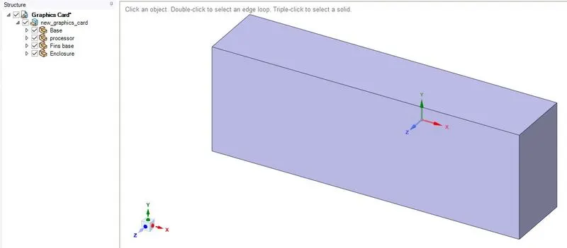
At the start of the simulation process, the made-up (Rough) geometry of the graphics card which also already includes an encloser was imported into the Space Claim. The various components involved in the geometry are highlighted with the orange rectangular boundary line which includes the base (circuit board), Graphics card processor, Fins attached to the processor, and other components.
Graphic card
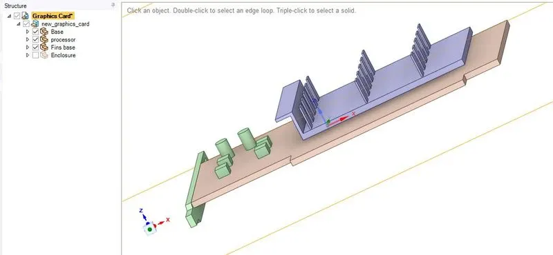
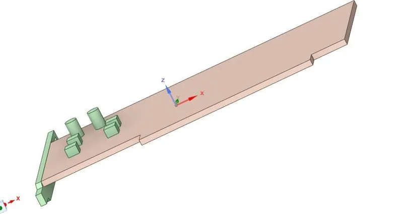
Base
Processor
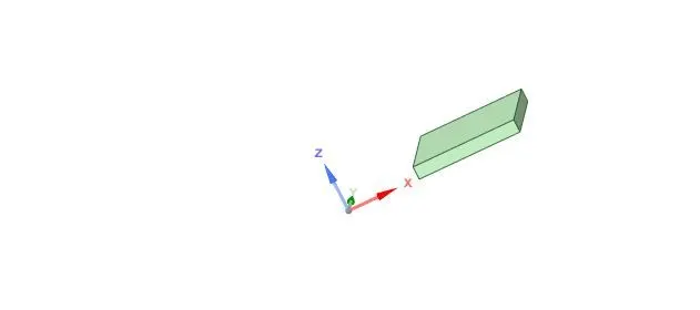
Fins
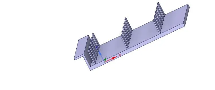
The geometry and flow domain consists of a flat circuit board with a heat-generating electronic processor chip and some other components connected to it. Heat is conducted through the source (processor), the board mounted on it and the fins attached to the processor. A stream of air flows over the fins, processor, and board, causing simultaneous cooling of the solid components and heating of the airstream due to convection. Thermal energy is also transported due to the complex flow field.
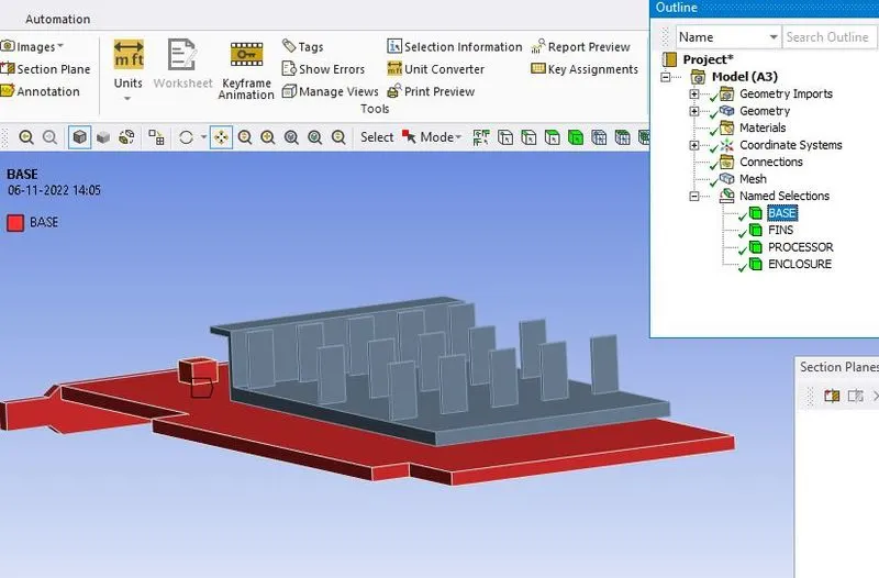
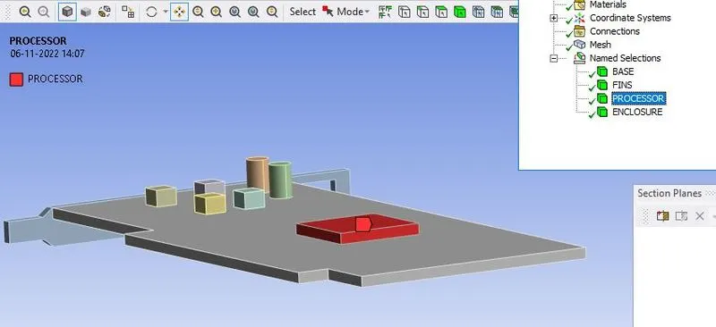
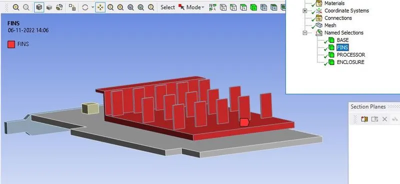
We start the mesh by naming the parts
1. Inlet
2. outlet
3. Wall
4. Fins
5. Base
6. Processor
Mesh setup:
1. Before generating a base mesh, let's name the different components of the graphic card so it is easier to find them while setting up fluent.
2. Base, processor, and fins are basic name selections that will help us in the simulation.
3. Click generate mesh to create a base mesh, body sizing can be applied for the 3 solid components.
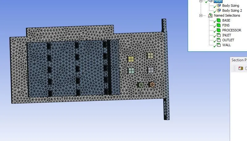
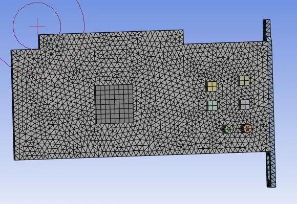
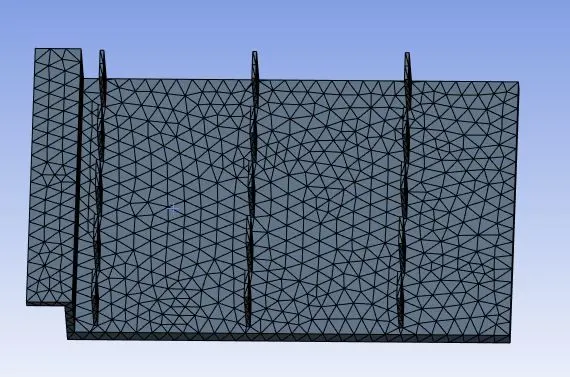
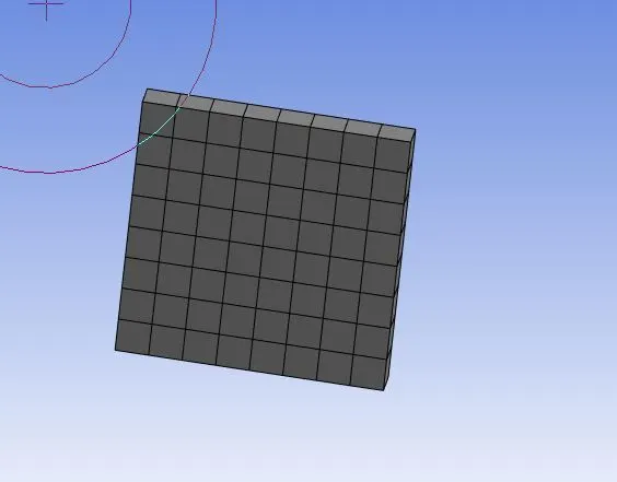
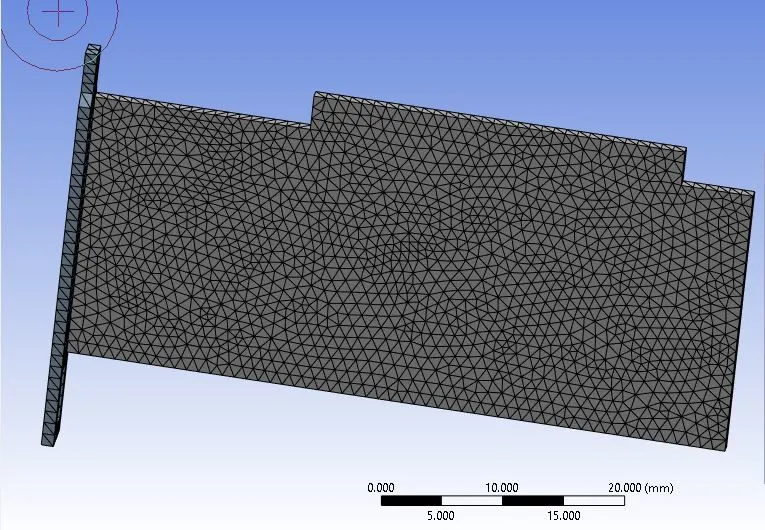
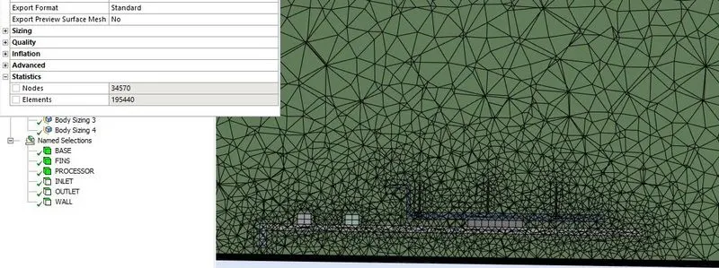
4. after creating body sizing for the 3 components, generate mesh as that it is considered as a base mesh having more than 1 lakh elements which helps us in finding accurate solutions.
5. After creating the mesh, exit the Mesh setup to simulate in fluent.
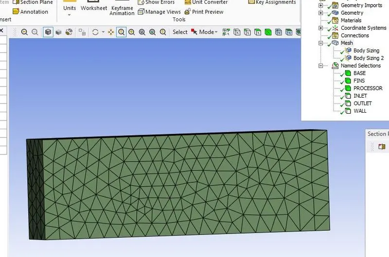
The generation of mesh over a graphics card circuit will show the following results.
Fluent setup:
Setting up the physics:
Setting up the physics for CHT analysis on a graphics card in ANSYS fluent.
In the Fluent settings, the type of solver is used as pressure based. Velocity formulation was set to absolute and the problem was simulated as considering steady-state simulation.
In this particular simulation, the temperature must be calculated so the energy equation needs to be enabled.
For this simulation, the k-omega turbulent model is considered which is best used for near-wall treatment. This is vital for this simulation as we expect the heat transfer coefficient calculated on the surfaces.
From the K-omega model, SST was selected as it provides a better prediction of flow separation than most RANS models and also accounts for its good behavior in adverse pressure gradients. It can account for the transport of the principal shear stress in adverse pressure gradient boundary layers. It is the most commonly used model in the industry given its high accuracy to expense ratio.
|
Solver Type |
Pressure-Based |
|
|
Velocity Formulation |
Absolute |
|
|
Time |
|
|
|
Models |
Viscous model: K-omega SST Energy model: On |
|
|
Material |
Fluid type: Air Solid-type: Copper : Silicon : Polystyrene |
|
|
Cell zones |
Fluid type: Air Solid: Cu, Si, Polystyrene |
|
|
Boundaries |
Inlet: Inlet velocity: 1 m/s Temperature = 300K Outlet: Outlet pressure = 0 |
|
|
Reference values |
Standard |
|
|
Initialization |
Standard |
Materials:
We are using different materials for all the component
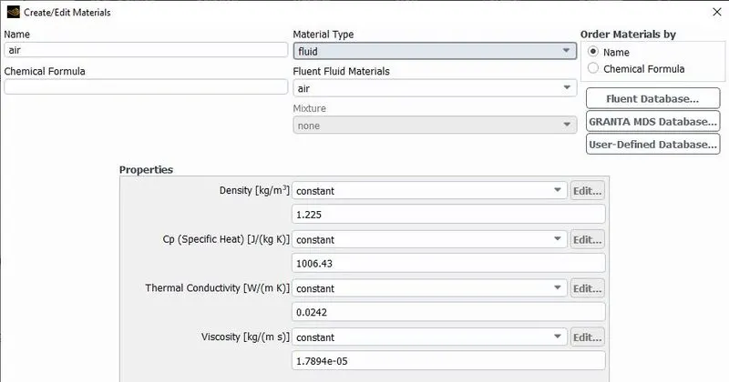
For fluid: Air
- Density = 1.225 kg/m^3
- Viscosity = 1.7894e-05 kg/ms
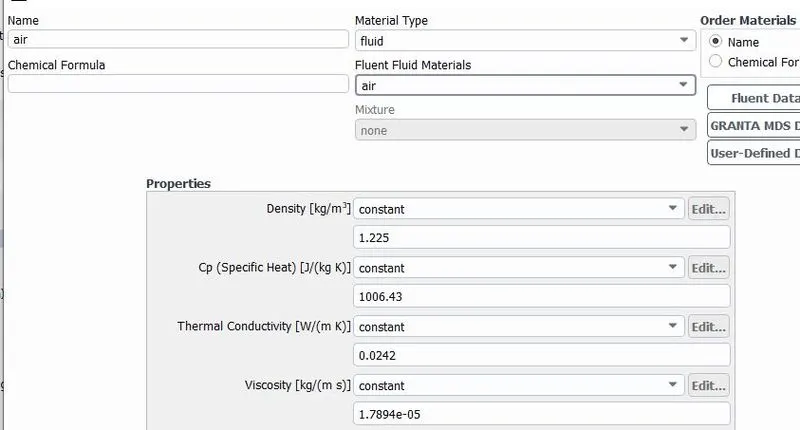
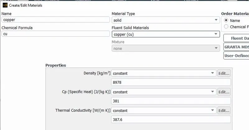
Copper is a good conductor of heat therefore it was added to assign it to fins.
For Fins: copper
- Density = 8978 kg/m^3
- Specific heat = 381 j/kg-k
- Thermal conductivity = 387.6 w/m-k
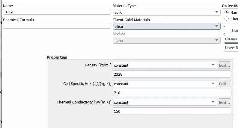
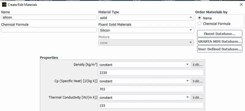
For Processor: Silica
- Density = 2328 kg/m^3
- Specific heat = 710 j/kg-k
- Thermal conductivity = 150 w/m-k
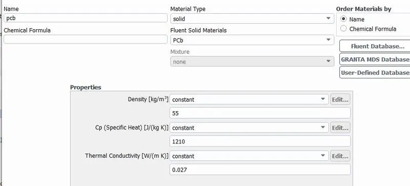
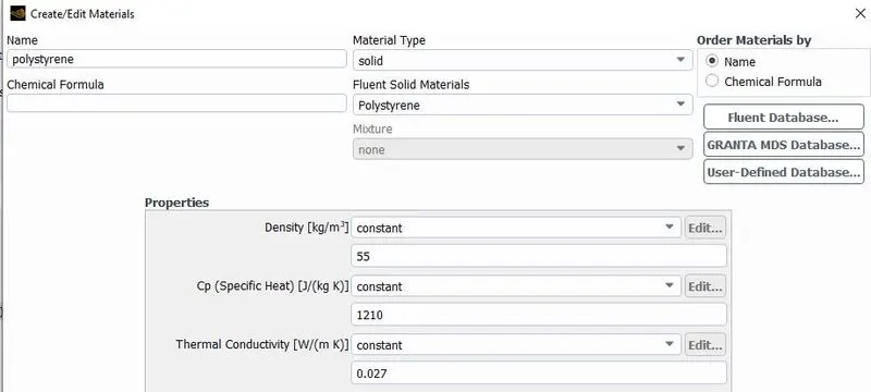
For Base: Pcb-Polystyrene
- Density = 55 kg/m^3
- Specific heat = 1210 j/kg-k
- Thermal conductivity = .027 w/m-k
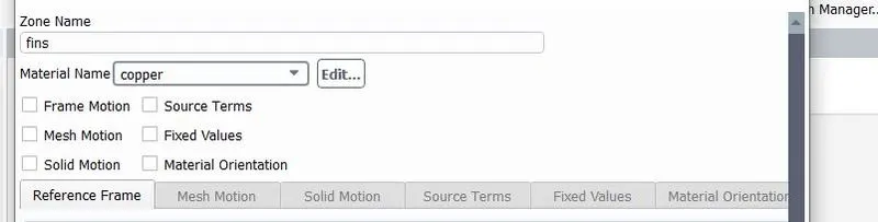
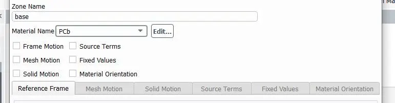
In cell zone condition material was assigned to their respective component as per portray in the below picture.
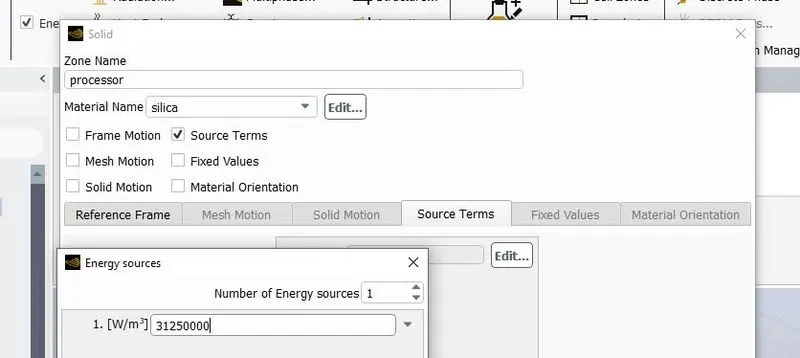
The Graphics card processor chip is the main heat source, hence, activate the source setting in fluent. Then, here, we have to define how much energy is released from the processor.
Usually, the power consumed by a processor is converted into heat energy. To calculate the heat generated on the processor which is = Power consumed divided by the total volume of the processor
Graphics Card Power (P) = 2 W
Volume of the card (V) = 8 x 8 x 1 = 64 mm^3
Heat Generated = P/V
The processor is assumed as the only source of heat.
The heat generated by the processor is 31250000 w/m^3
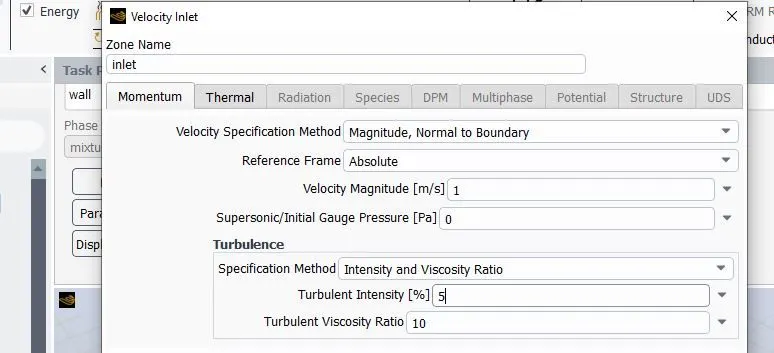
Inlet velocity was taken as 1 m/s
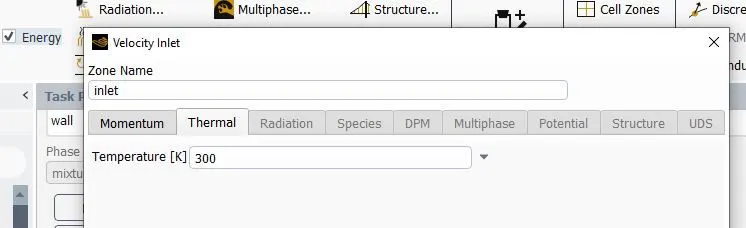
Normal inlet air temperature is considered as 300K.
After setting up the materials and assigning the fluid and solid zones separately we run for 500 iterations and see that the solution converged.
The first one was the baseline simulation for getting a rough idea and results for the further final simulations. The next two simulations were performed to check the mesh dependency of the problem setup.
Part 1: 3 different simulations with 3 different mesh sizes.
Case 1: Base Mesh (Coarse)
Global mesh setting of element size = 10 mm
Fins size: 1 mm
Processor: 0.6 mm
Base: 1 mm
Number of elements = 195440
Fins
Processor
Base
Cut section of geometry
Case 1 Results:
Residual plots
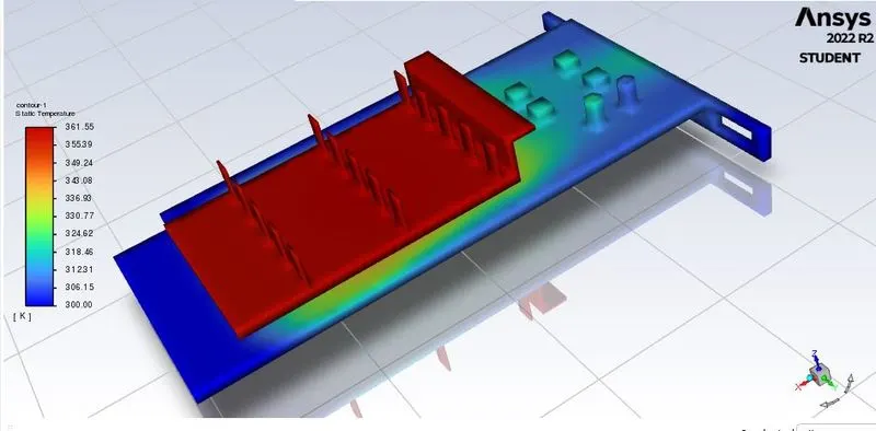
The temperature on the Graphic card
Post Processing:
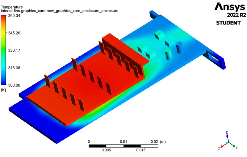
Temperature contour global
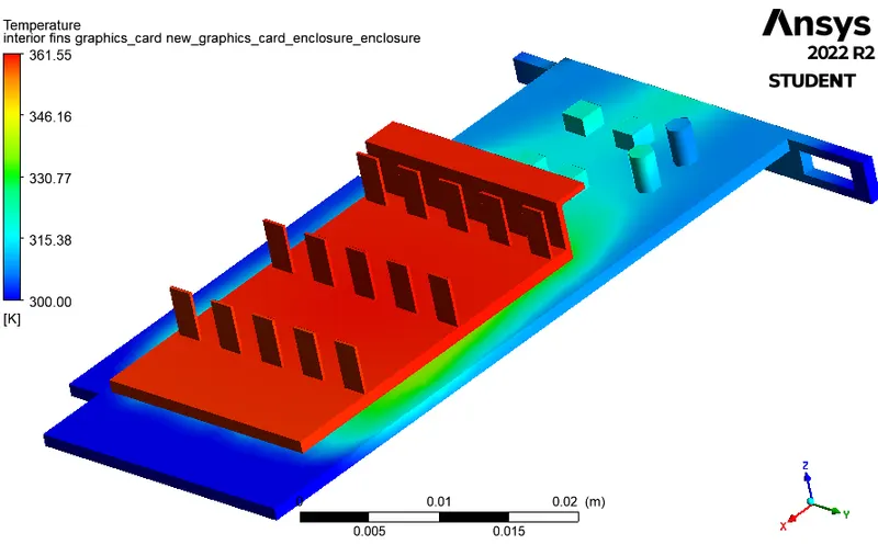
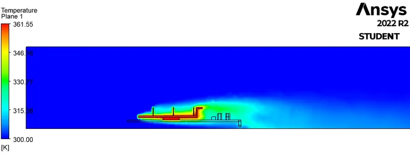
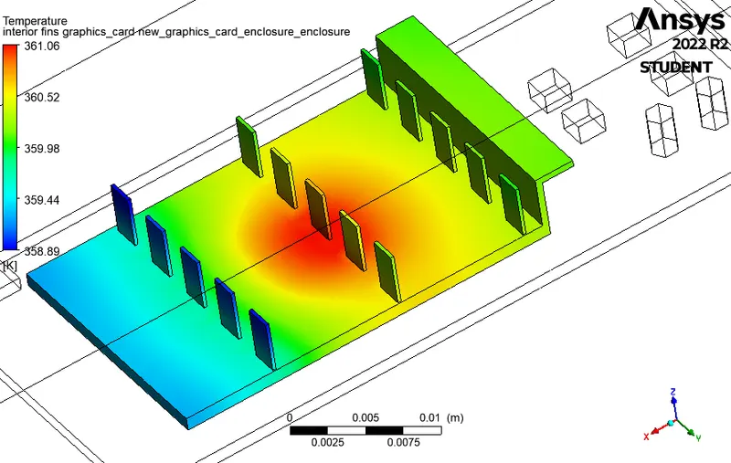
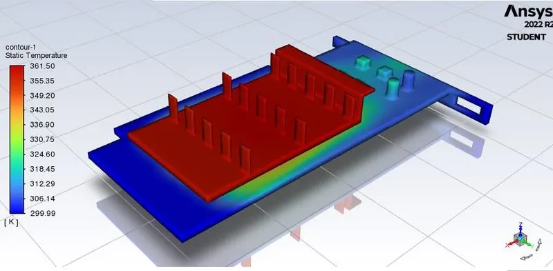
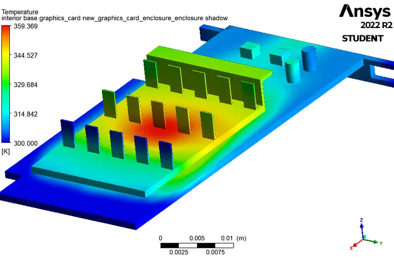
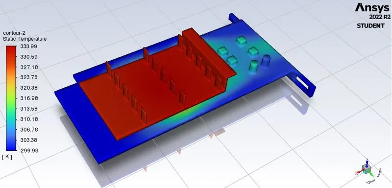
The max temperature reached by the system is 361.55 kelvin. The PCB doesn't conduct the heat to a great extent so it remains around 300 kelvin. Also, there appears to be a local hotspot in the center of the fin base.
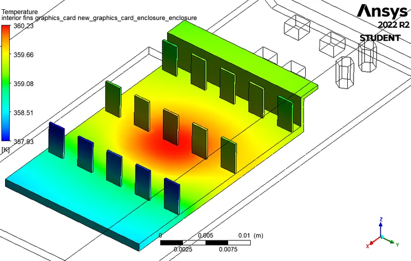
Temperature contour local
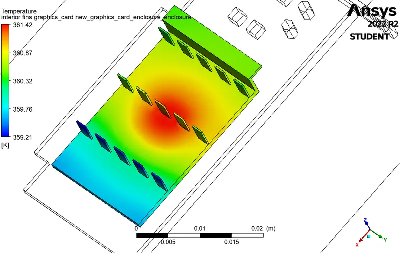
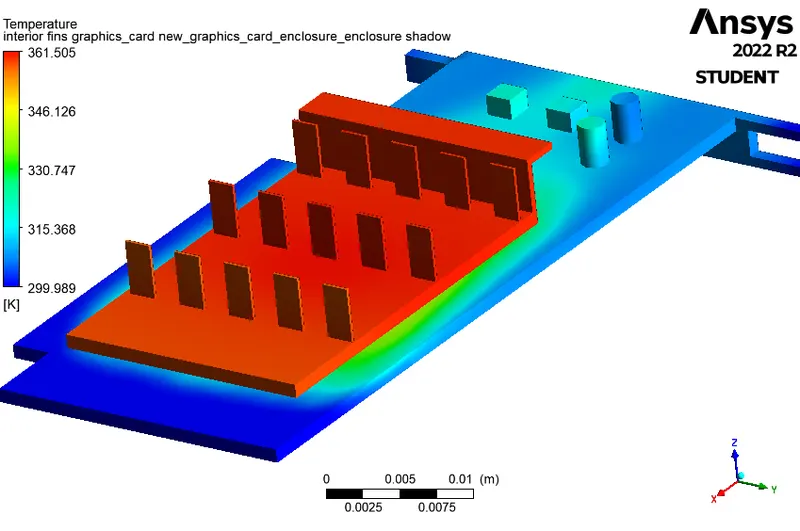
It can be seen that the fins at the front are cooler than the ones behind. This happens because the cold air first hits the front fins, it gets heated up and goes to the next fin. Hence, the next fins can't give it enough heat as the difference in temperature is lower between solid and fluid.
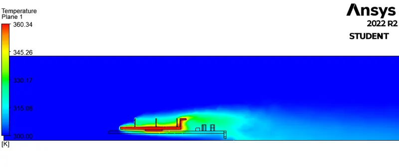
Temperature plane
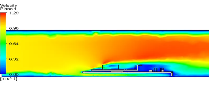
Velocity plane
Velocity plane zoom in
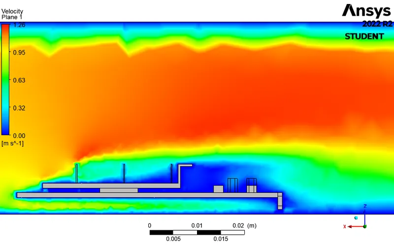
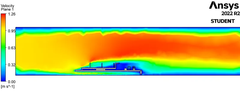
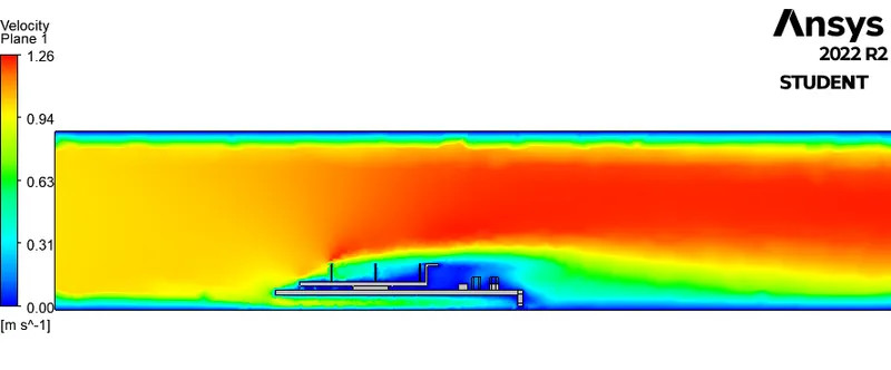
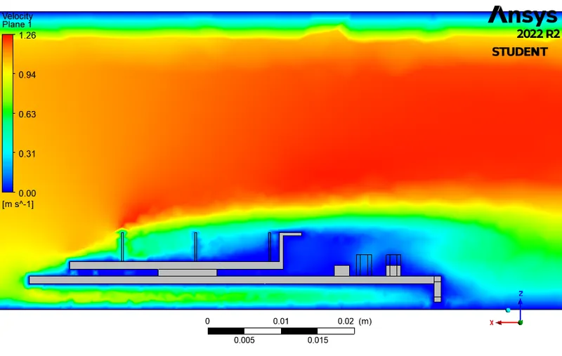
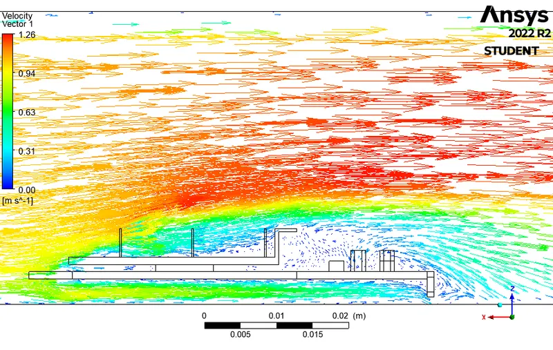
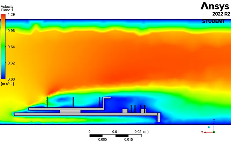
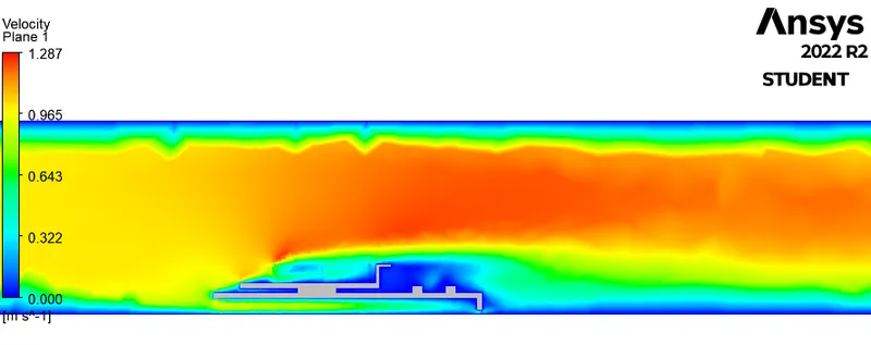
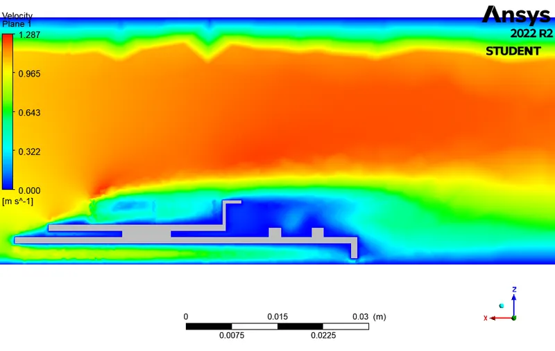
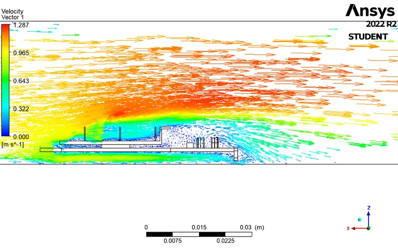
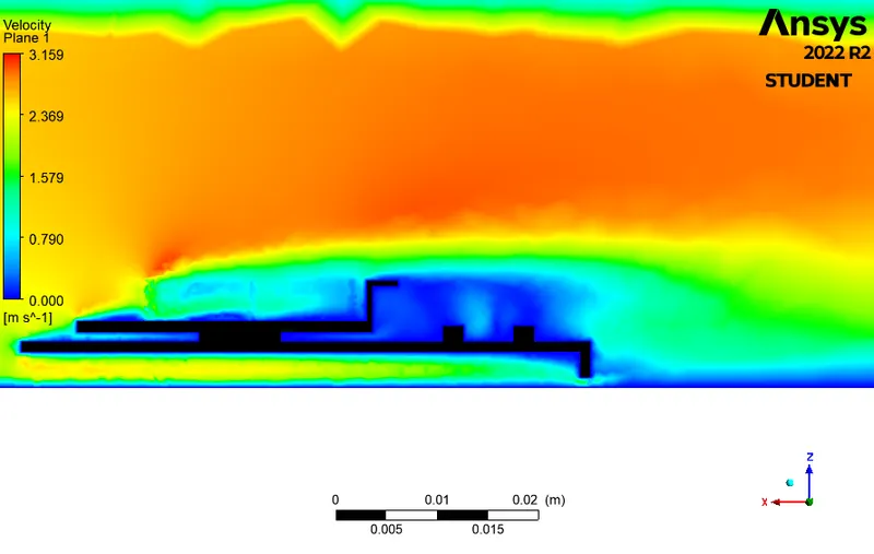
The flow has a dead (wake) region behind the fins. It should be seen correctly through a vector plot.
Vector plot
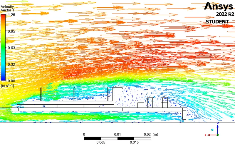
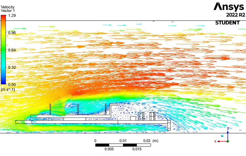
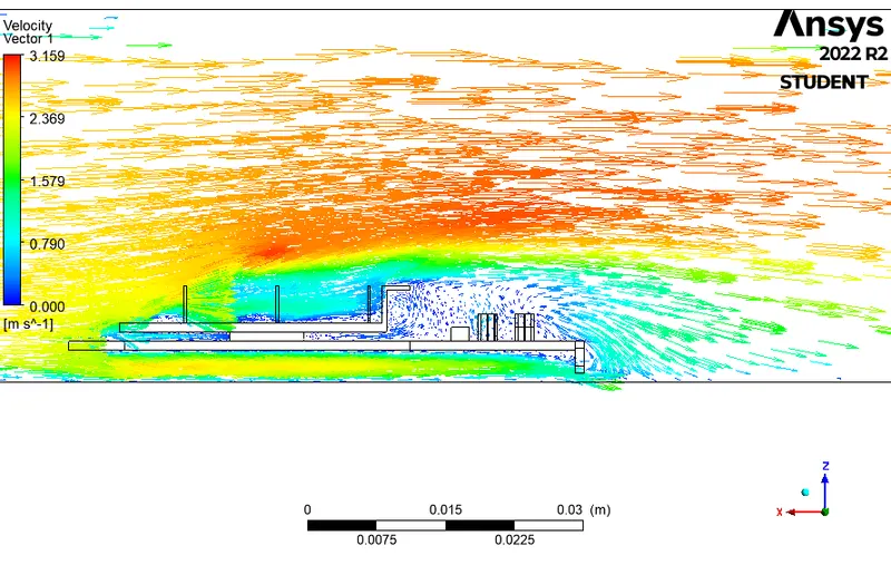
There are 3 recirculation regions formed and their velocity is less than 0.3 m/s. So, it is important to look at flow over this region using streamlines.
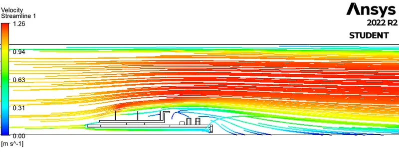
Velocity streamlines
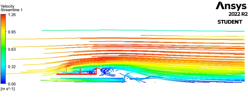
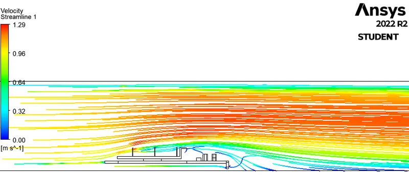
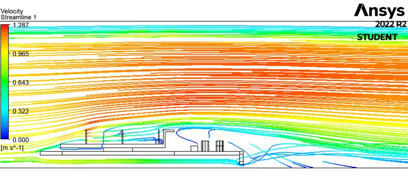
It is seen that the components behind the fin plate receive high-temperature air with low velocity (<0.3 m/s). If any component generates heat over that region, it would not cool down faster. If a component doesn't generate heat, the air would heat that component. So, either way, the heat will stay in that region, causing problems for the components to present there. So, the processor must be placed at last in the flow direction.
The streamlines coming from below get heated by the processor and rise above from the sides thus heating the sides of the fins and its base.
The streamlines show the formation of two giant recirculation regions, formed due to the air flowing from the sides to the middle of the fin structure's back.
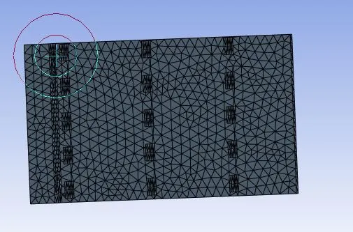
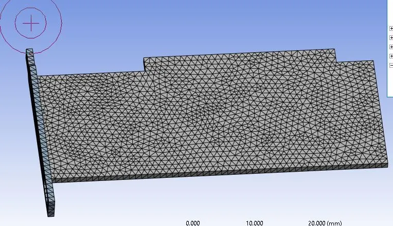
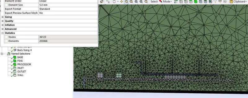
Case 2: Medium refined mesh
Global mesh setting of element size = 5 mm
Fins size: 0.8 mm
Processor: 0.4 mm
Base: 0.9 mm
Number of elements = 203866
Fins
Processor
Base
Cut section of geometry
Case 2 Results:
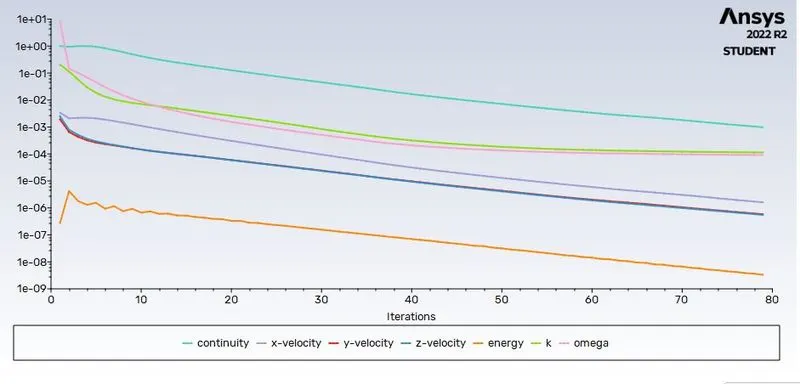
Residual plots
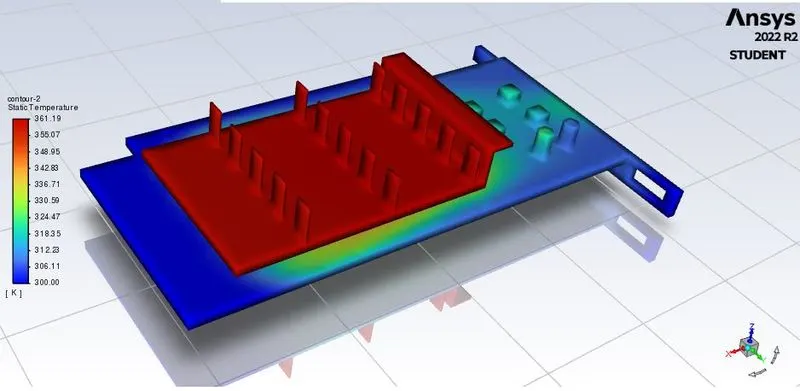
The temperature on the Graphic card
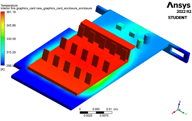
Post Processing:
Temperature contour global
Temperature contour local
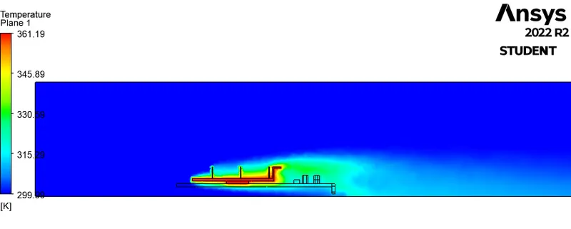
Temperature plane
Velocity plane
Velocity plane zoom in
Vector plot
Velocity streamlines
Now here we have refined the setup and made it to 314130 cells just near the academic license limit. The finer mesh will let us give precise results around the edges and the heat transfer coefficient. This is what we made the mesh accordingly:
Case 3: Refined mesh
Global mesh setting of element size = 7 mm
Fins size: 0.6 mm
Processor: 0.2 mm
Base: 0.7 mm
Number of elements = 314130
Fins
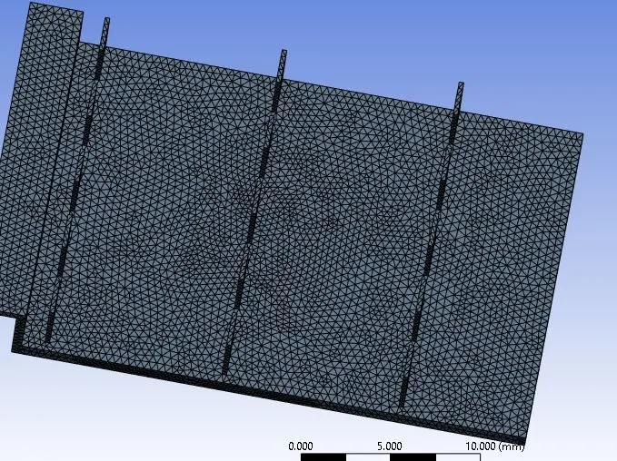
Processor
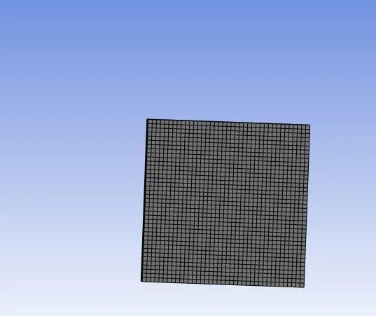
Base
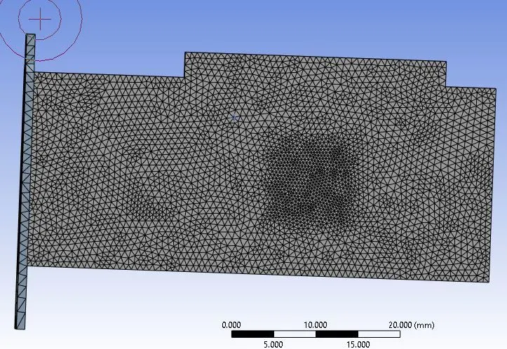
Cut section of geometry
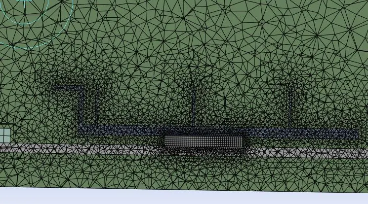
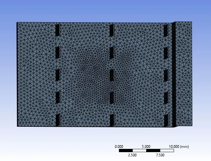
As you can see here when the element size is reduced the mesh gets finer and more importantly around the microprocessor and the base components, the mesh is structured by itself as we apply the body sizing mesh tool to MICROPROCESSORS and FINS.
Case 3 Results:
Residual plots
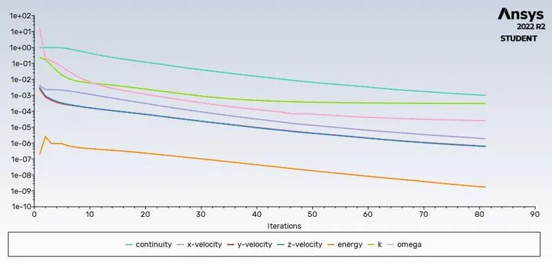
The temperature on the Graphic card
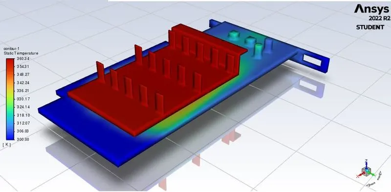
Post Processing:
Temperature contour global
Temperature contour local
Temperature plane
Velocity plane
Velocity plane zoom in
Vector plot
Velocity streamlines
In the first three simulations, we ran a solution for 1m/s velocity to check the mesh independence. And with each case we got results in a very close range, hence, the mesh is dependable. Therefore, for further simulations, for velocities 1 m/s, 3 m/s, and 5 m/s, the same duplicate setup and refined mesh were used.
Part 2: 3 different simulations with 3 different velocities
We are more interested in the thermal energy transfer from the Microprocessor to the Aluminium fin where it cools with airflow and this is where our turbulence model also plays a vital role, well there's not much of a difference in its varietals, but this tells us how heat transfer takes place and this is the only 2 body in the GPU where the temperature is at highest, and we can see that in our previous different mesh cases fin and microprocessor CFD-post results. That's why here we are using refined mesh.
Mesh size
Global mesh setting of element size = 9 mm
Fins size: 0.6 mm
Processor: 0.2 mm
Base: 0.8 mm
Number of nodes = 87514
Number of elements = 472819
Fin
Processor
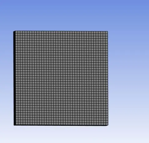
Base
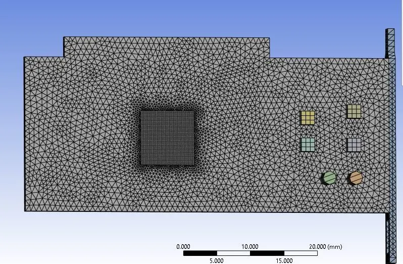
Cut section of geometry
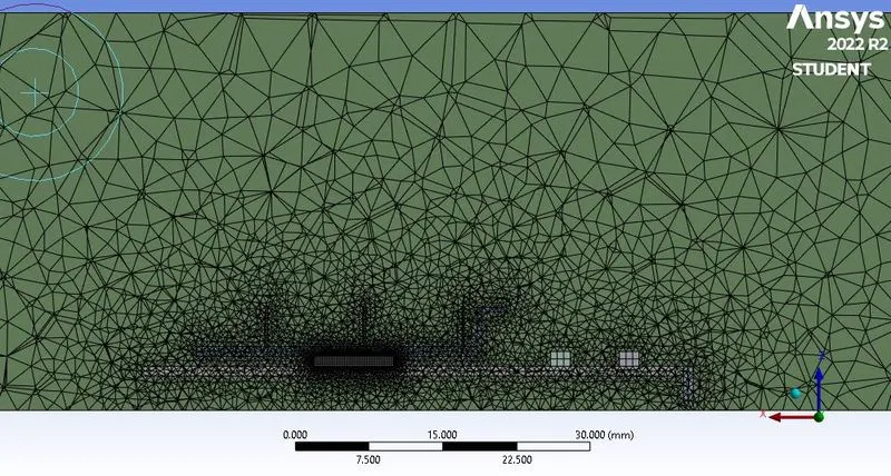
As you can see here when the element size is reduced the mesh gets finer and more importantly around the microprocessor and the base components, the mesh is structured by itself as we apply the body sizing mesh tool to MICROPROCESSORS and FINS.
Material used
Fin material
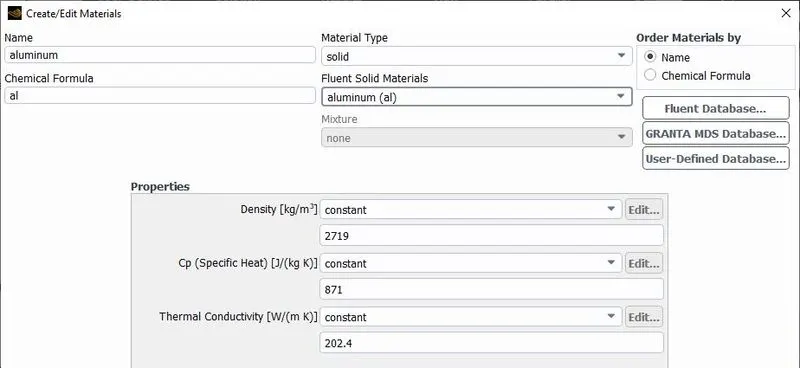
Processor material
Base material
Fluid material
Solver: Steady
Type: Pressure Based
Turbulence Model: k-Omega(SST)
Materials: Different materials are used for each part, some of which are custom created
Graphics Card Power (P) = 2 W
Volume of the card (V) = 8 x 8 x 1 = 64 mm^3
Heat Generated = P/V
The processor is assumed as the only source of heat.
The heat generated by the processor is 31250000 w/m^3
Setting up the source terms:
For this case, we consider that our processor is a source term and it generates heat.
So, for setting up the source term go to Zones - Cell zones - and click on the processor for editing which is in the Solid.
After that select the material to Silicon & click on the source terms to enable it and set the energy source to 1.
The simulation setup is the same as that selected for the initial cases. Only the output of the simulation will change because of the change in the inlet velocities.
Case 4: Inlet velocity was taken as 1 m/s
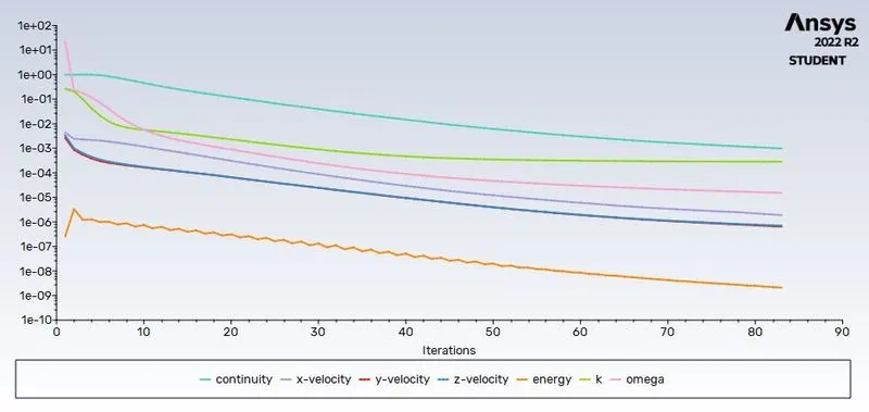
Residual plots
The temperature on the Graphic card
Surface heat transfer coefficient
Average Temperature
Post Processing:
Temperature contour global
Temperature contour local
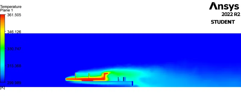
Temperature plane
Velocity plane
Velocity plane zoom in
Vector plot
Velocity streamlines
Case 5: Inlet velocity was taken as 2.5 m/s
Residual plots
The temperature on the Graphic card
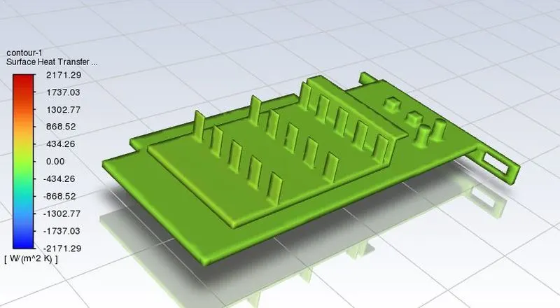
Surface heat transfer coefficient
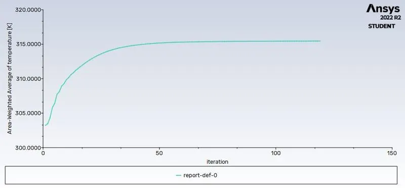
Average Temperature
Post Processing:
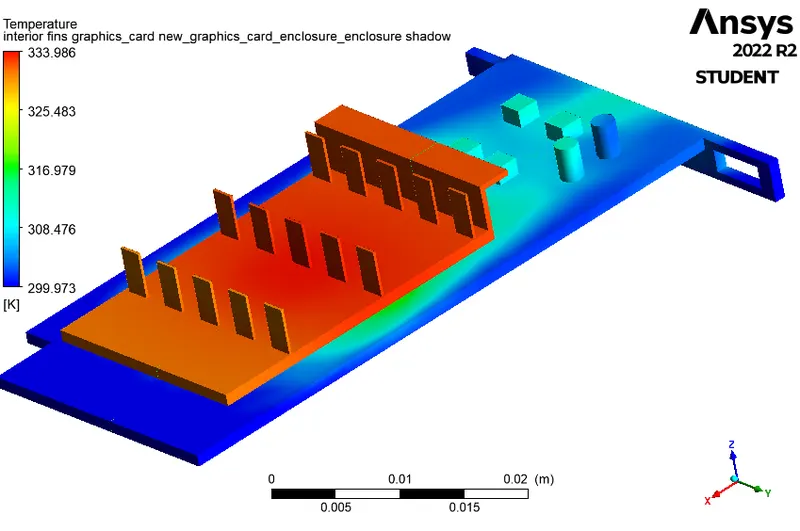
Temperature contour global
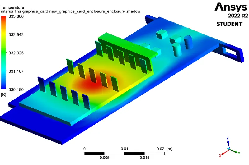
Temperature contour local
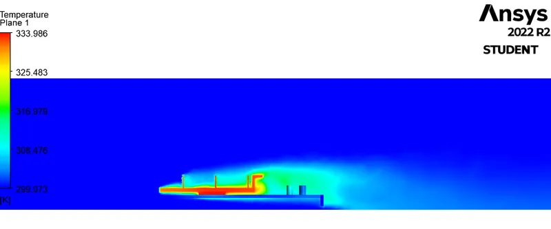
Temperature plane
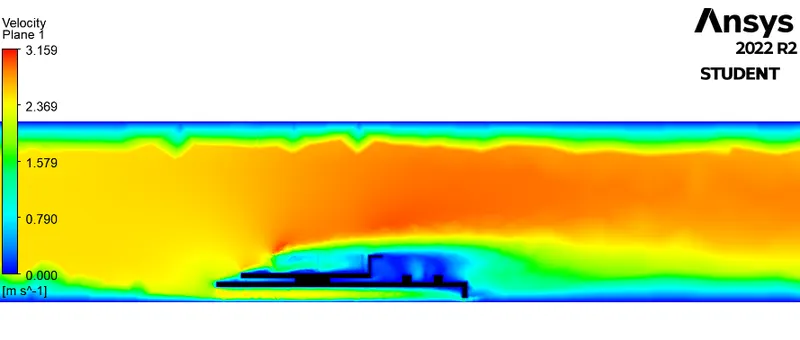
Velocity plane
Velocity plane zoom in
Vector plot
Velocity streamlines
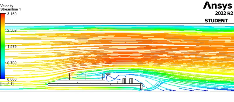
Case 6: Inlet velocity was taken as 5 m/s
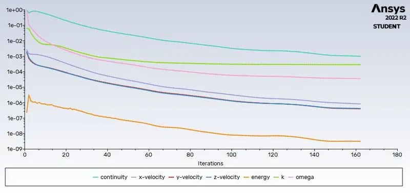
Residual plots
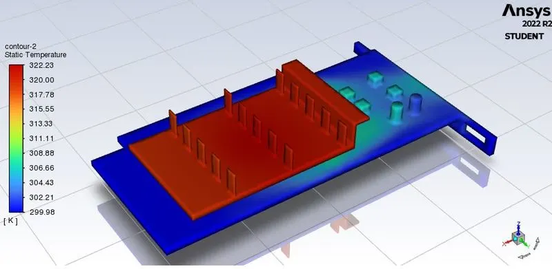
The temperature on the Graphic card
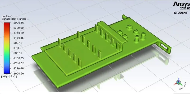
Surface heat transfer coefficient
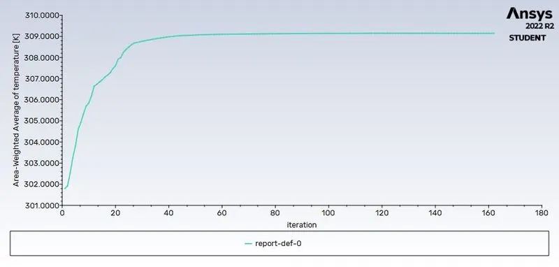
Average Temperature
Post Processing:
Temperature contour global
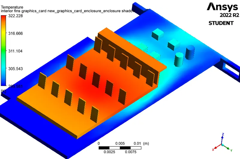
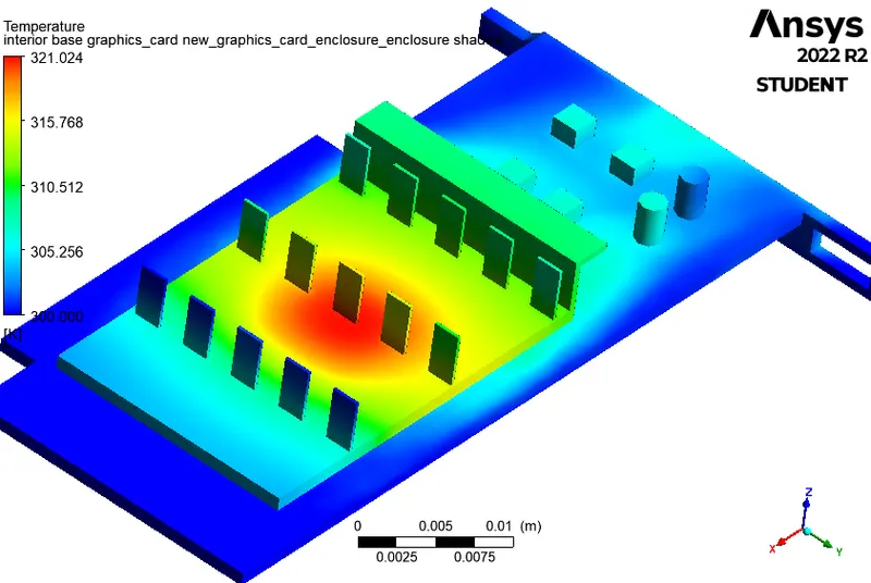
Temperature contour local
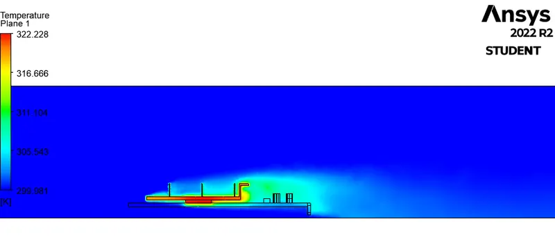
Temperature plane
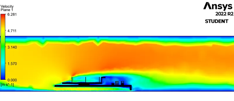
Velocity plane
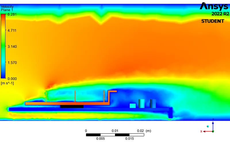
Velocity plane zoom in
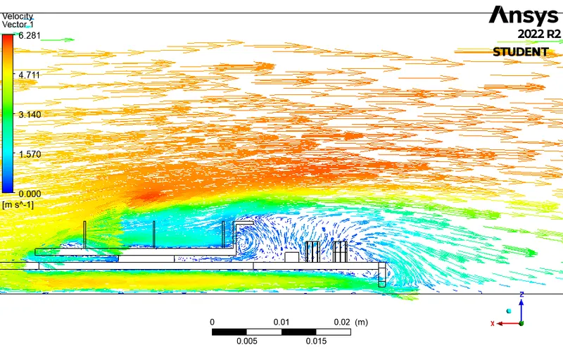
Vector plot
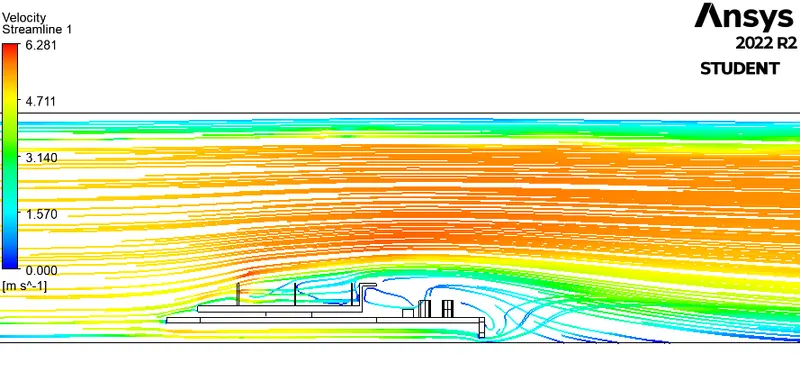
Velocity streamlines
Results:
| Velocity (m/s) |
Area-Weighted Average Temperature (Kelvin) |
HTC at Fin (W/m^2-k) |
Maximum Temperature (Kelvin) |
Maximum Velocity (m/s) |
| 1 | 330 | 256.94 | 361 | 1.2 |
| 2.5 | 315 | 258.35 | 333 | 3.1 |
| 5 | 309 | 262.49 | 322 | 6.2 |
A converged solution for the given sets of input was observed based on repetitive plots in the Residual plot. The processor acted as a source of heat input and thus one of the hotspots for such a study.
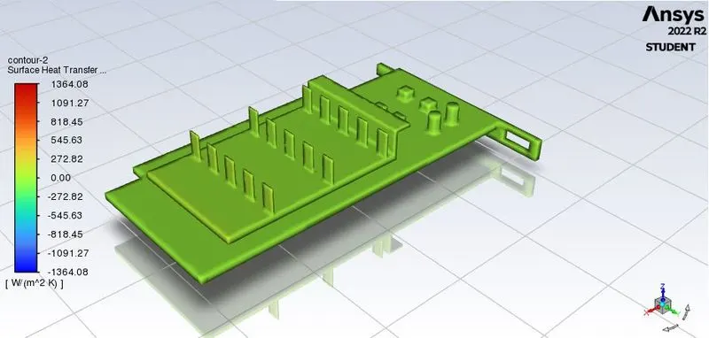
With an increase in velocity, we saw a considerable drop in temperature and a substantial rise in heat transfer coefficient which shows that high-velocity air can be an effective mode of heat dissipation in graphics card
From the temperature distribution, we can see hotspots in the fin and base near the surface that is in contact with the processor. Based on the thermal conductivity of the material this temperature is distributed accordingly amongst the component. We see a few high-temperature zones on the fin away from the processor depicting their high susceptibility to heat due to their geometry.
Also, the difference in baseline and refined mesh is considerable and thus we can conclude that more refined mesh provides a better solution and can be used in optimizing the design for such applications. From the residual plot, the change in the gradients is very small with which we can conclude that the solution has converged.
From the temperature plot of the coarse mesh, the high-temperature points are found at the fins, processor, and base area near the processor. As the wall heat transfer coefficient is a wall phenomenon and fins dissipate a large amount of heat which results in a higher heat transfer coefficient but the coarse mesh heat transfer for fins and other components in the graphics card has the same values. Hence refinement of mesh is done for fins and base of the fin and base of the graphic card to calculate the wall heat transfer coefficient at the fins and base.
The high-temperature regions are found at the center of the fins, base, and processor walls. With further iterations, the temperature is distributed to other regions in the graphics card in the direction of the inlet airflow. Conduction occurs where there is a contact region between the solids in this case it is between the processor and fins and the processor and base. Convection occurs when the heat generated in the components of the graphic card is removed by the inlet airflow. The maximum temperature in the components is inversely proportional to the inlet airflow velocity. With the increase in the airflow velocity, the heat removal process by convection is faster. And also recirculation of air (vortex) at appropriate places will increase the heat transfer efficiencies hence greater amount of heat is removed by convection.
Conclusion:
As the number of elements increases accurate results of temperature distribution are obtained.
From the above table, it is fairly notable that, the net temperature of components of graphics cards decreases with an increase in inlet velocity.
Hence it can be inferred that a higher inlet velocity results in better cooling and lower average temperature thus keeping the components safe from damage.
Furthermore, it can be observed that the temperature of components increases as the inlet velocity decreases from 5 m/s to 1m/s, also proving that higher velocity results in better cooling.
Higher velocity in a particular region means a higher Reynolds number. That’s why the heat transfer coefficient in that area is the highest, which means the maximum amount of heat transfer is taking place from fluid to the solid in that region. This also results in a higher temperature of solids in that location.
To identify the Hotspots we have studied and analyzed several cases for the temperature and HEAT transfer coefficient. so we know that the most potential Hotspots are around the Fin base and the whole microprocessor.
Heat transfer coefficient is a function of properties of the fluid at film temperature, temperature difference, temperature coefficient, and buoyance force et, hence, mesh resolution near walls usually has the biggest impact on numerical results.
For the turbulent models, we have to take care of the assumptions and the boundary conditions you put in the program. The mesh is a very important parameter to get nice results so we have to refine it in the important place of our drawing.
Some factors should be considered and the most significant is the turbulent boundary layer. If we are using any kind of low Reynolds turbulence model considering enhanced wall treatment (as your K-omega SST model), so we need to make sure that we stay in the laminar sub-layer region where velocity profiles are assumed to be laminar and viscous stress dominates the wall shear which means
Mesh/ grid dependency test is very important to get confidence over results.
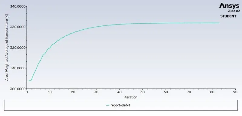
Another way to confirm whether results are converged or not is by observing the Average temperature of the solid. As the table flow after a particular time, the temperature of solids also maintains its temperature in a very minimum constant range which shows the final solution is achieved.