Week 6 - CHT Analysis on a Graphics card
Aim :- To perform Conjugate Heat Transfer (CHT) analysis on a Graphics card
Objective :-
- To understand the CHT anlysis , how to analysis conjugate heat transfer on a model by performing steady state solver
- To become experienced about verious meshing and their effect on the result ( heat trnsfer coefficient , temperature , velovity)
- Also know about how to find the max temp and htc , etc
Theory of the project :-
What is Conjugate Heat Transfer - Conjugate heat transfer is a type of heat transfer analysis between solids and fluid(s). This type of heat transfer includes both convection (between fluids) and conductive (between solids) heat transfer, as well as both forced and natural convection.
Why CHT analysis is used - Conjugate heat transfer (CHT) analysis is used to predict heat transfer acculately by simultaneous solving all the relevant solid and flow field heat transfer processes, for example: conduction through solids.
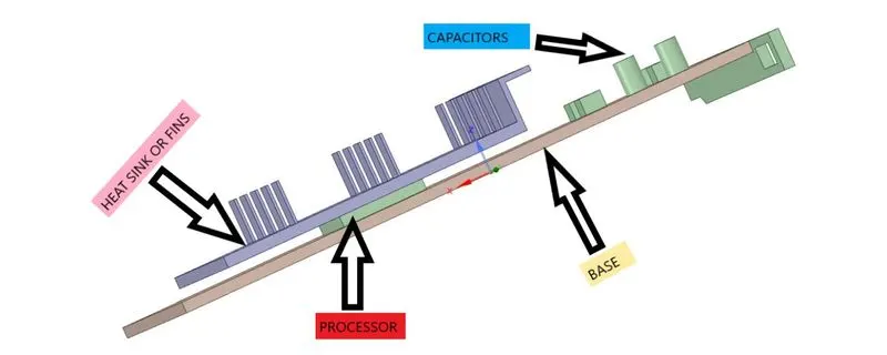
Modelling and problem solving approach:
1. Start the anys fluent workbanch
2. First import the geometry in spaceclaim
3. Meshing - baseline and refinement and named selection
4. Energy on
5. Steady state simulation using viscous K epsilon model
6. Creating material
7. Boundary condition
8. Standard initializing
9. Run Fluent solver
10. Post-processign and animation plots
Importing the object in spaceclaim :-
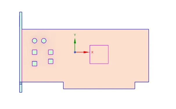
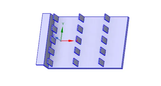
As the object is already given , just need to import the object un spaceclaim and enabled the share topology to share the information between diffrence bodies .
Base Fins
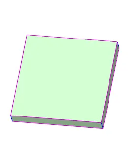
Processor
Final geometry after creating the plane and enable the share topology in workbench
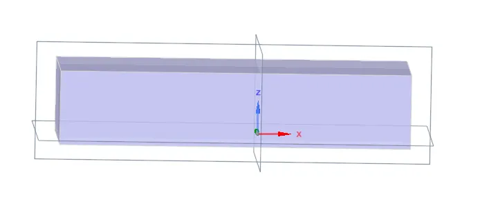
This is our final geometry . Now we can go ahead with meshing the geometry .
Meshing :
- Open the meshing console.
- Click on the mesh and select generate mesh option.
- Now a basic mesh pattern will be created.
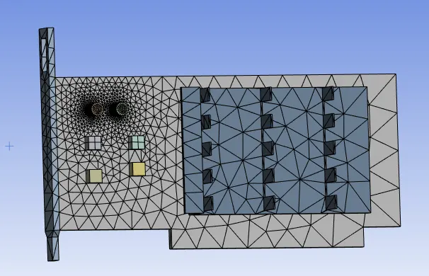
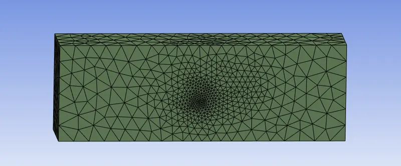
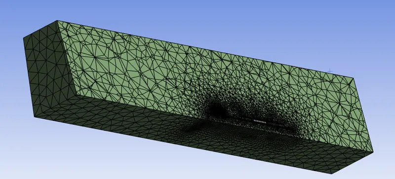
- Now we will run a baseline mesh having default size of around 10 mm . We go to mesh size and put the desired value>> click on generate mesh tab.
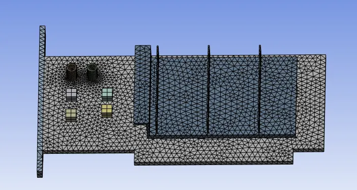
- Now on the next step we will refine the mesh size by 6 mm and will go for body sizing for the fins, pcb , processor with 0.4 mm respectively.
Mesh settings:
Global mesh setting of element size = 10 mm and for refine mesh 6 mm
1) PCB body sizing
element size = 0.4 mm
capture curvature - yes
2) Processor body sizing
element size = 0.4 mm
capture curvature - yes
3) fins body sizing
element size = 0.4 mm
capture curvature - yes
Default mesh
Pre processing set-up:-
Materials & their properties: (Ref [3],[4])
1) Fins --> Aluminium
Standard aluminium is available in Fluent database.
Density = 2719 Kg/m^3
Heat capacity = 871 J/KgK
Thermal conductivity = 202.4 W/mK
2) Processer --> Silicon
Since the silicon is not available in Fluent's solid database, I had to define it
Density = 2330 Kg/m^3
Heat capacity =703 J/KgK
Thermal conductivity = 153 W/mK
3) PCB (Polystyrene)
Since the FR4 is not available in Fluent's solid database, I had to define it
Density = 55 Kg/m^3
Heat capacity = 1210 J/KgK
Thermal conductivity = 0.027 W/mK
4) Fluid --> Air
Standard air is available in Fluent database.
Density = 1.225 Kg/m^3
Heat capacity = 1006.43 J/KgK
Thermal conductivity = 0.0242 W/mK
Viscosity = 1.7894e-05 Kg/m-s
Setup:
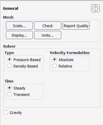
Steady state analysis
Energy on - as we are looking for temperature
Solver - pressure based
Turbulence model - k-e model
Inlet velocity = 1 m/s , 3 m/s and 5 m/s for different case
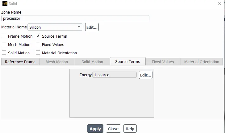
Source Term in Processor : 31250000 w/m^3.
To consider for heat generation in the processor many standard values were referred to from the internet & catelogues of Graphic card manufacturing companies like Nvidia. The power consumption lies anywhere between 40 to 120 watts from low end to high. However our gpu model's size is a little smaller than standard ( refer in the reference) . So the power Consumption considered is 2 watts.
The volume of model processor is 64 mm^3.
Hence calculating the Source Term as such : `2div(64*10^-9)`
Case 1 with Baseline mesh setup :
Meshing (Size = 10.289 mm)
Inlet velocity = 3 m/s
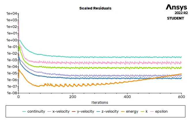
Iteration to converge
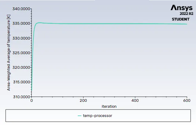
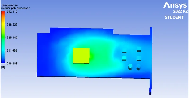
Temperature plot of interior processor
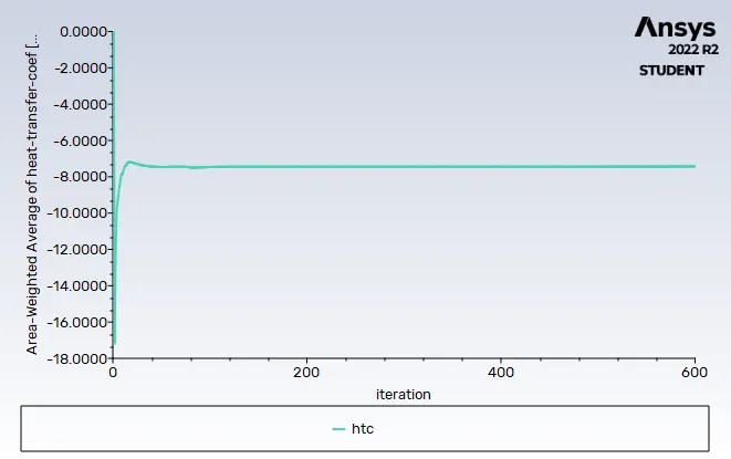
Heat transfer coefficient plot
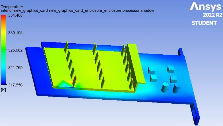
Temperature contour of processor
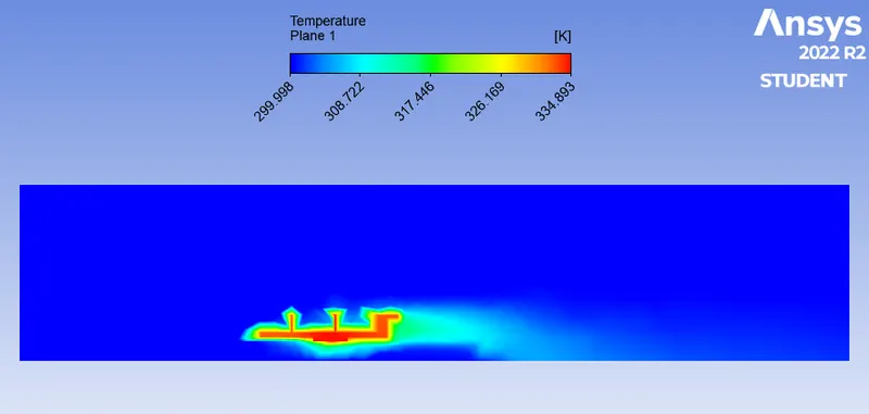
Temperature contour on zx plane
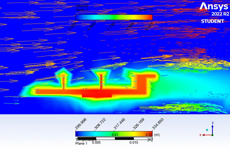
Velocity vector and foe plan we have coloured by temperature
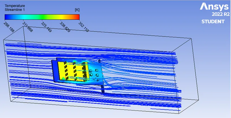
Temperature streamline
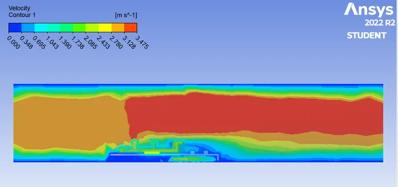
Velocity contour
Case 2 with Refined mesh setup :
Meshing (Size = 6 mm, body sizing= 0.4 mm)
Inlet velocity = 1 m/s
Iteration to converge
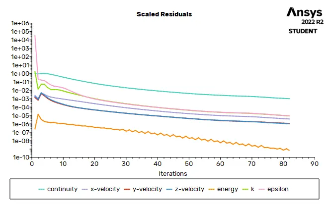

Solution is converged at 82 solution
Temperature plot of interior processor
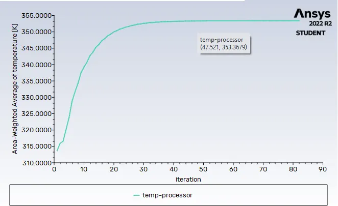
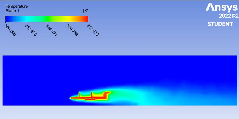
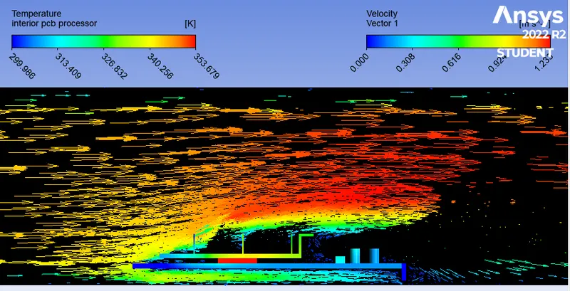
Potential Hot spots on the model
The pcb is the hot spot as the processor is directly attached over it. 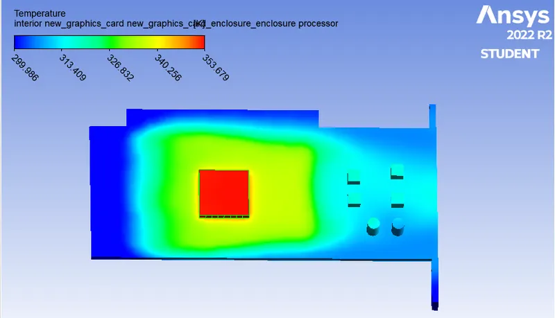
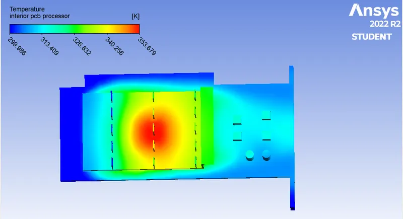
Temperature contour on zx plane
Velocity vector
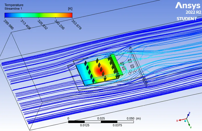
Temperature streamline
Case 3 with Refined mesh setup :
Meshing (Size = 6 mm, body sizing= 0.4 mm)
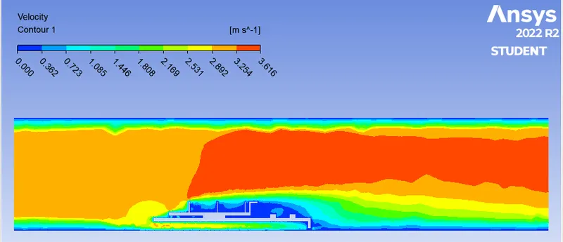
Inlet velocity= 3 m/s
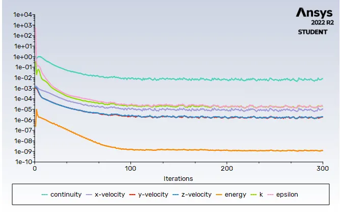
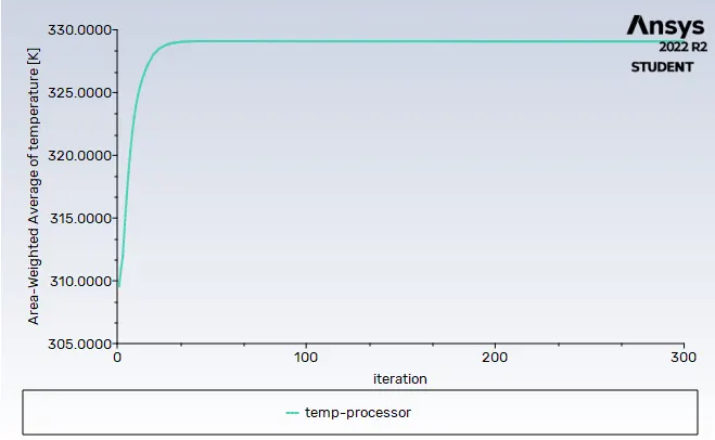
Iteration to converge
Temperature plot of interior processor
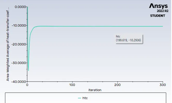
Heat transfer coefficient plot
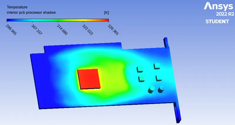
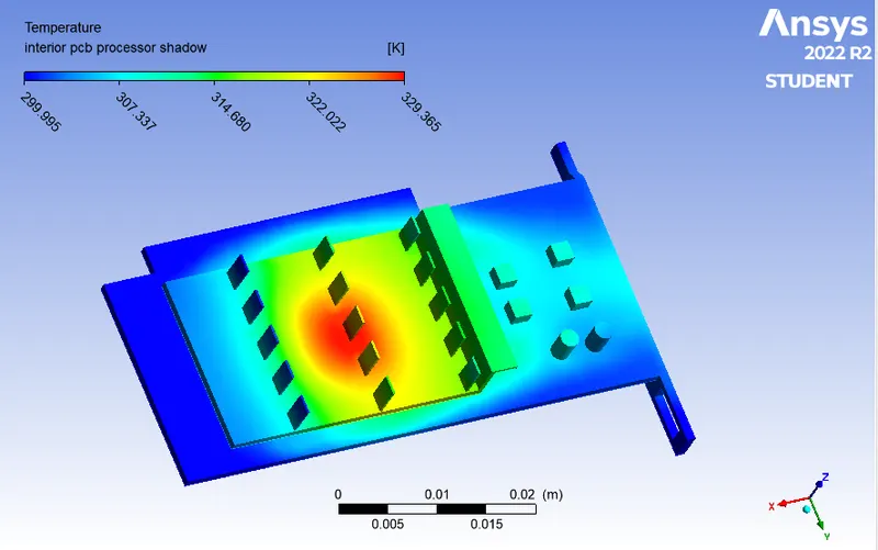
Potential Hot spots on the model
The pcb is the hot spot as the processor is directly attached over it.
Velocity vector
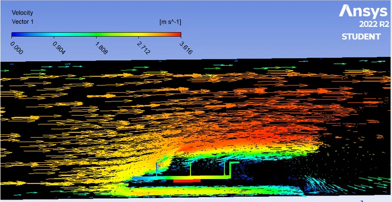
Velocity contour on zx plane
Temperature streamline
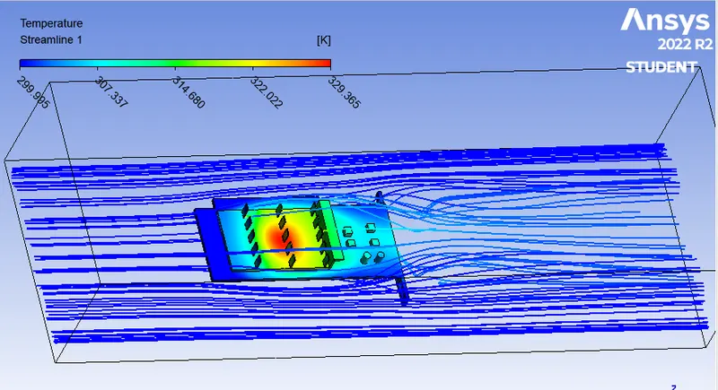
Case 4 with Refined mesh setup :
Meshing (Size = 6 mm, body sizing= 0.4 mm)
Inlet velocity= 5 m/s
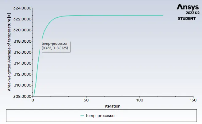
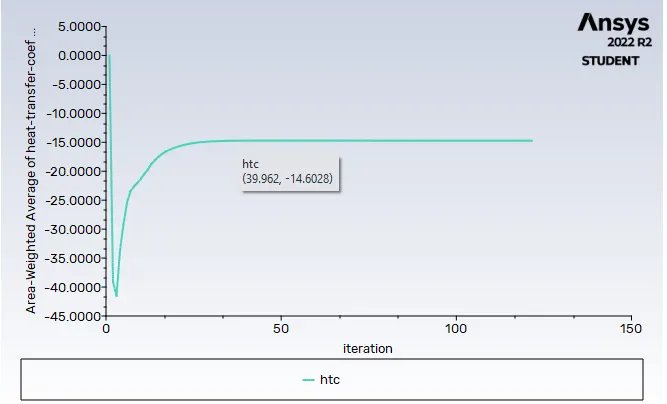
Iteration to converge
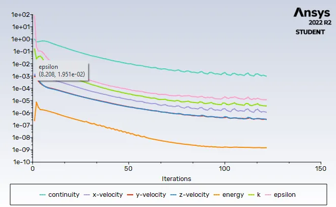

Solution is converged at 122 solution
Temperature plot of interior processor
Heat transfer coefficient plot
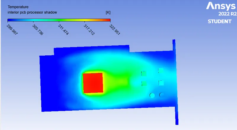
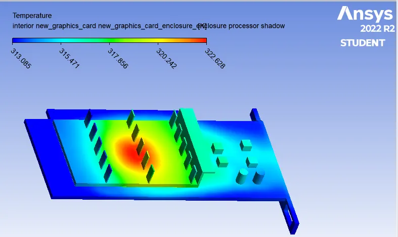
Potential Hot spots on the model :
The pcb is the hot spot as the processor is directly attached over it.
Velocity vector
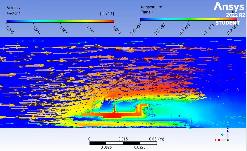
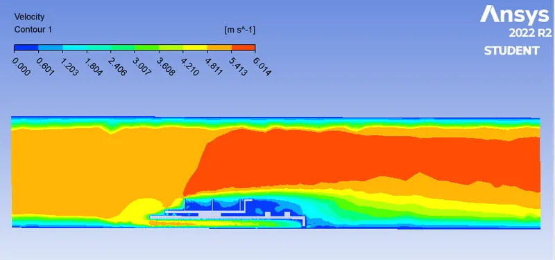
Velocity contour on zx plane
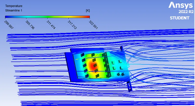
Temperature streamline
Observation :- Here to understand the difference we have given same velocity for baseline and refine mesh
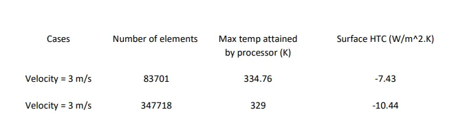
1. You can see that for fine mesh max temperarure attained by the processer has decreasing and heat transfer coefficient has also decresing .
We have given different inlet velocity as 1 m/s , 3 m/s and 5 m/s to see the diffrence in tmperature and contour plots
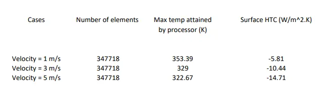
As the velocity is increasing the max temperature and htc attained by processor decreasing gradually .
Conclusion :-
1. We conclude the solution convergence by first observing the residuals where all the equations converged . Secondly the desired results where achieved as we expected it. i.e the idea in mind of what the cht simulation results would prove was infact observed in every iteration of the solution which leads us to conclude a fully converged solution.
2. The max temperature attained by the processor will always vary, like it increased when the air flow was less and decreased when it was more. hence proper cooling of such electronic devices is necessary for efficient functioning.
3. The conjugate heat transfer study allowed us to peak into electronics heat distribution, working and many conceptual clearance which are before theoretically verified in hand calculations or text book principals.
4. Heat transfer coefficient is something which changes with materials used, inlet velocity hence engineers are very picky about the materials used in these cards as they are so compact, the need to provide higher heat dissipation and improving performance directly results in earning more from customers. Thus heat sinks like fins, other shorter heat extending devices etc are carefully manufactured for this very purpose.
5 CHT study helps in identifying hotspots of the model in thermal analysis, these hotspots once discovered, gives the engineer the ability to make changes in the model where necessary and improve its thermal efficiency and performance.
6. Proper meshing has extremely important advantages as we observed from cases having significant differences in terms of maximum temperature.