Week 6 - CHT Analysis on a Graphics card

CONJUGATE HEAT TRANSFER ANALYSIS ON GRAPHICS CARD

Aim:

To determine the hotspots of a graphic card, the various heat transfer coefficients, there by predicting the durability and efficiency of the component.

Introduction:

A heat transfer analysis involves the calculation of the temperature distribution and flow of heat flux under thermal loads. Both steady-state and transient conditions are simulated. The study of transport phenomenon concerns the exchange of momentum, energy and mass in the form of conduction, convection and radiation. These are the three types of heat transfer involved in various types of materials.

Conjugate Heat Transfer analysis:

A conjugate heat transfer is the simulation between solid and fluid domains by exchanging thermal energy at the interfaces between them. The prediction analysis takes place simultaneously in both solid and fluid boundary. The solid boundary is characterized by stationary material particles, while the fluid boundary is characterized by the moving particles.

A CHT analysis can predict heat transfer through conduction, free or forced convection and radiation heat flows simultaneously between solids and fluids. The wall heat transfer coefficients and local derivatives are calculated within the model, which is an advantage over the empirical calculations.

The application of a CHT analysis is in the Heating, ventilation, air-conditioning and refrigeration environment. The key engineering applications include effective heat transfer, energy saving, appropriate heat transfer coefficient formulation etc.

A computer graphic card:

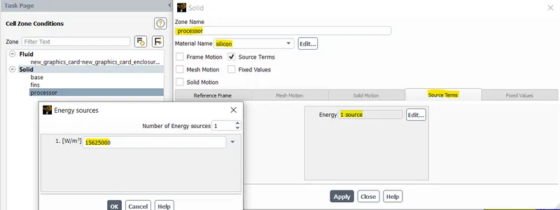
A graphic card is a integrated chip with the function of display adaptor or video card installed within most computing devices, to display graphical data with high clarity, colour, definition and overall appearance. The main component is the processor mounted on a base with other electronic components. Fins are provided above the processor to increase the efficiency of the heat sink. Silicon, Copper and plastic are the materials used for processor, fins and the base correspondingly. 15625000 is calculated as the heat source coming out of the processor. An enclosure is created around the component to provide the fluent environment.

Procedure:

Step 1: Setting up the geometry in Space Claim

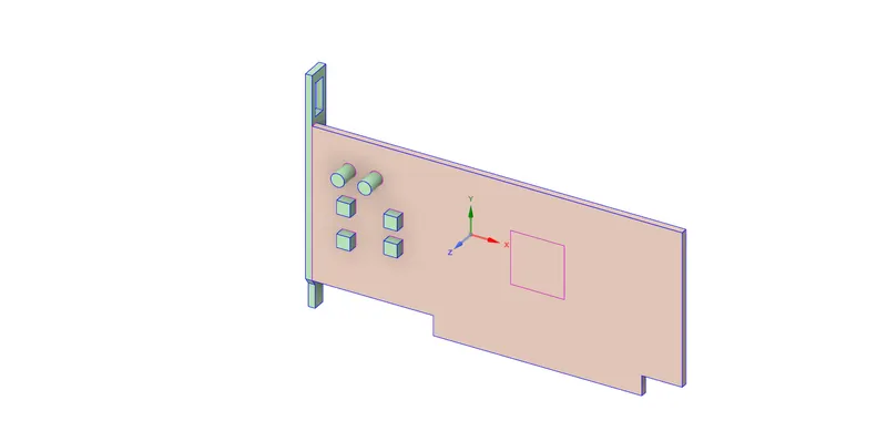
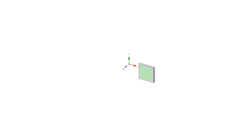
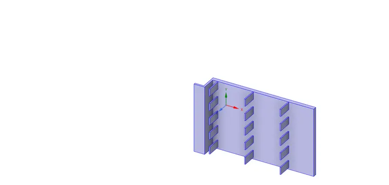
The parts of the graphic card include a processor mounted on a base, with fins on top for heat radiation.

Processor base with components

Processor

Fins above processor

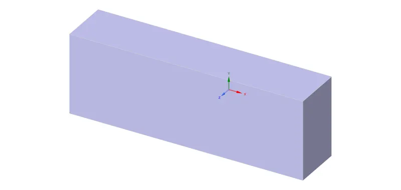
An enclosure is designed around the component to maintain a fluid environment and for easy simulation.

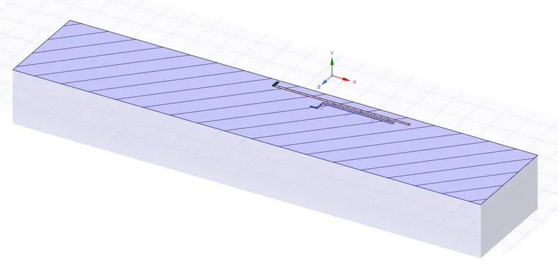The geometry is checked for interference, extra edges and component distributions.

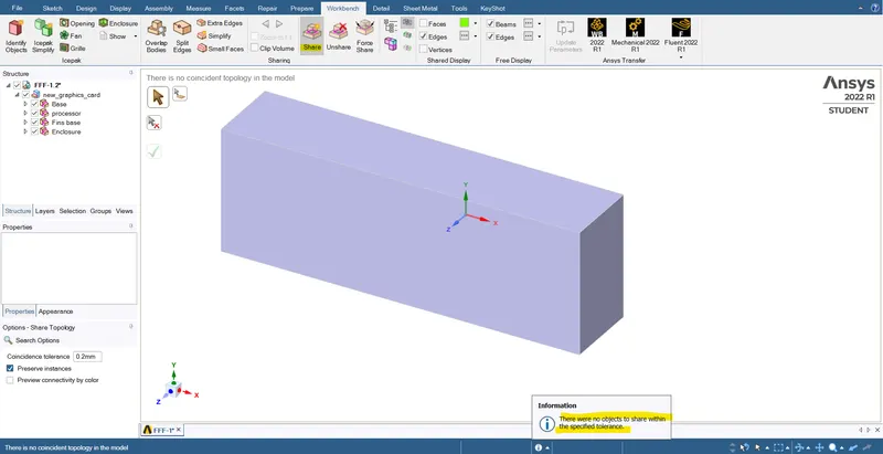
Finally, the geometry is checked for shared topology and updated to the mesh component.

Step 2: Meshing

Various components of the geometry are given different element size owing to the necessity of the application.

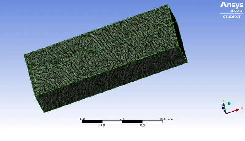
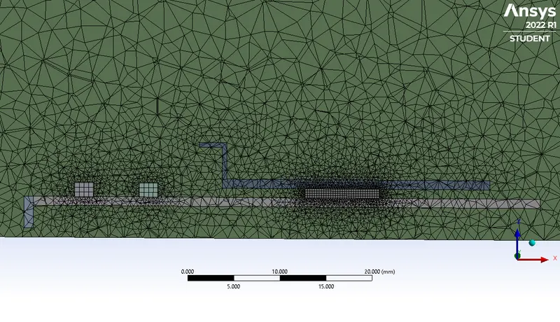
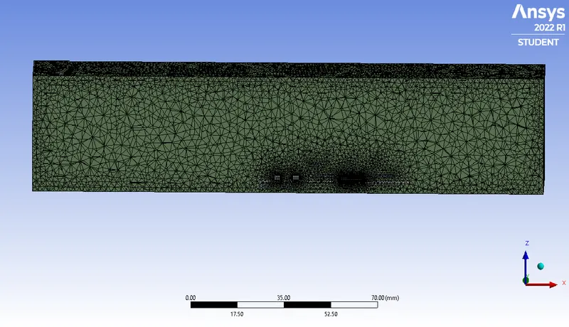
Fins, processor, base and the enclosure are given different sizes and with 3 body sizing methods, all are tetragonal majored cells with a conformal meshing property.

Fins, Body sizing 0.5mm

Processor, Body sizing 0.25mm

Components of base, Body sizing 0.5mm

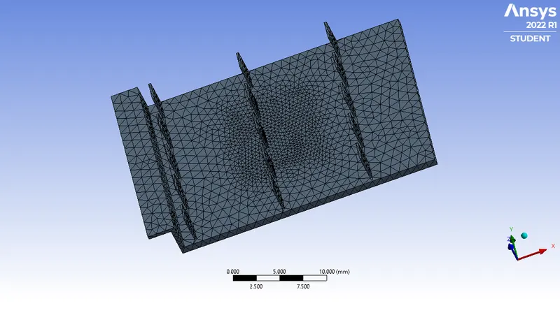
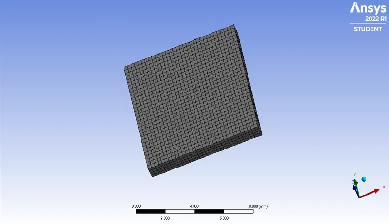
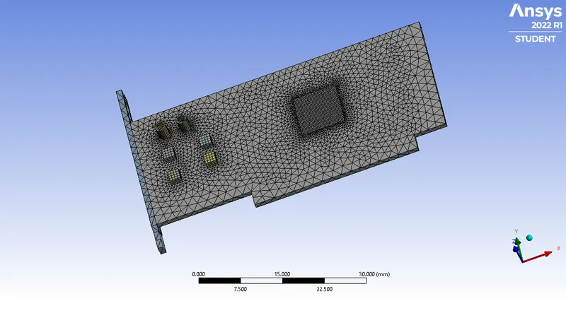
The enclosure and the base of the processor are given sizes of 2mm and 1mm respectively as there are more surface area and the accuracy can be met with this size.

Step 3: Setting up the fluent domain

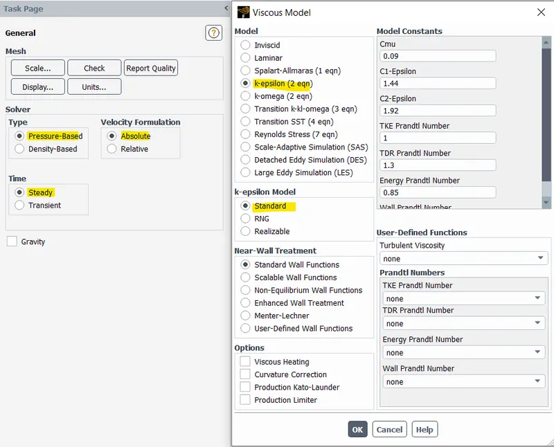
The basic solver settings are set to steady, pressure based K-epsilon model.

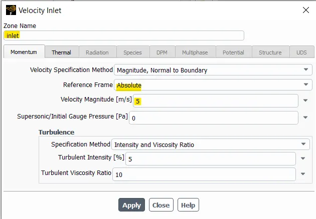
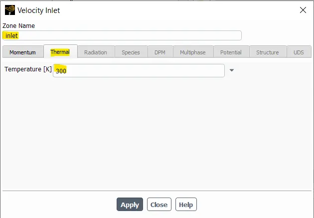
The boundary conditions are set for momentum and thermal inlet conditions.

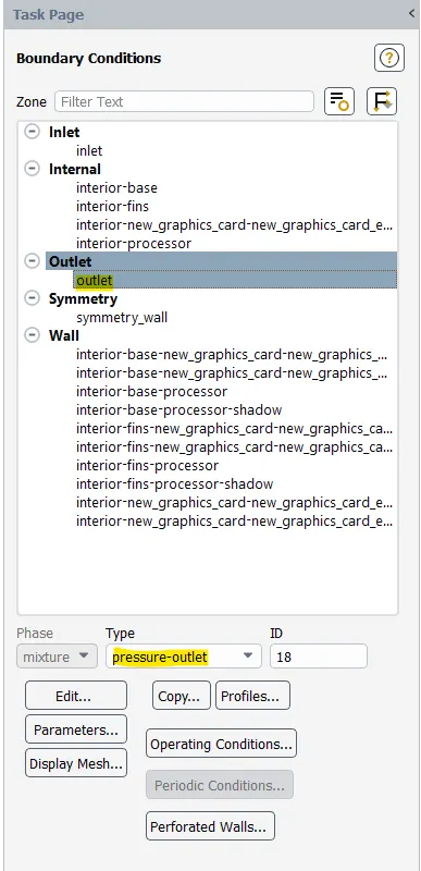
The pressure outlet and symmetry wall conditions for the enclosure is given respectively.

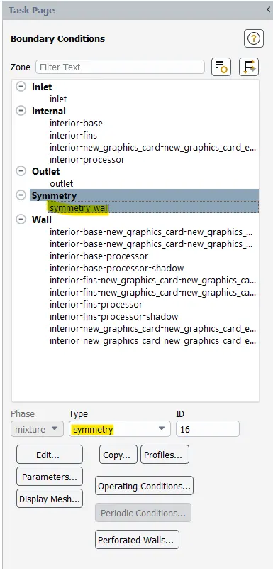
The material properties are created for the necessary materials needed in the simulation.

	Processor	Processor base	Fins	Enclosure
Material	Silicon	Plastic(High Density Polyethylene)	Copper	Air
Density (`(kg)/m^3`	2330	940	8978	1.225
Thermal conductivity (`W/(mK)`	156	0.4	387.6	0.0242
Specific heat `J/(kg.K)`	628	1500	381	1006.43

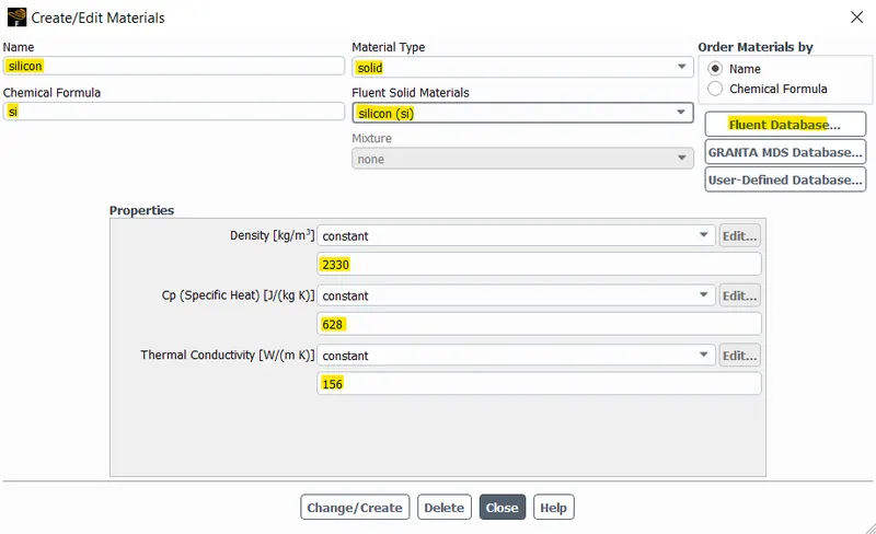
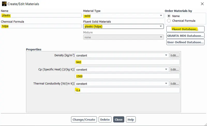
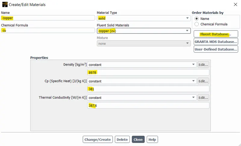
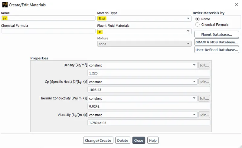
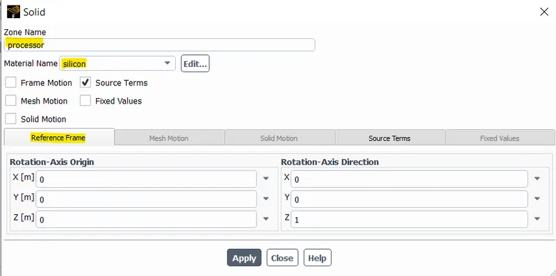
The materials for the components are assigned in the cell zones, for the processor, processor base, fins and the enclosure.

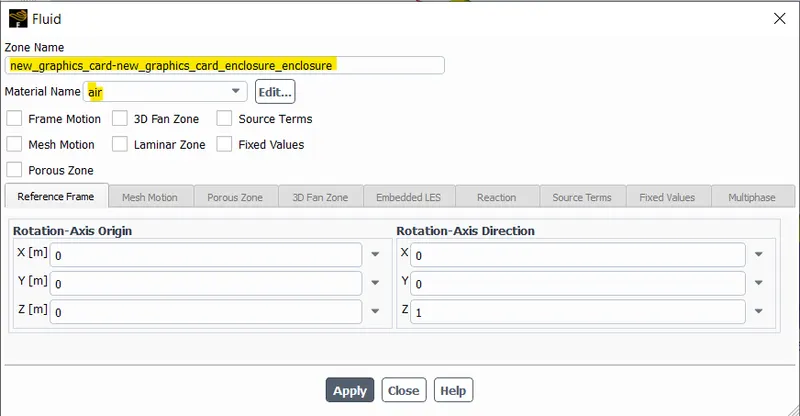
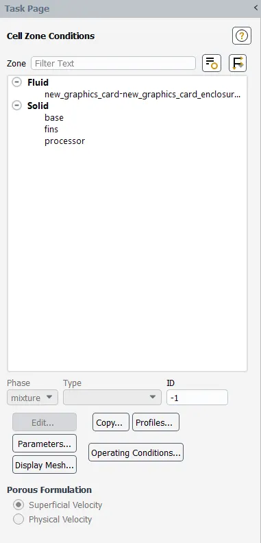
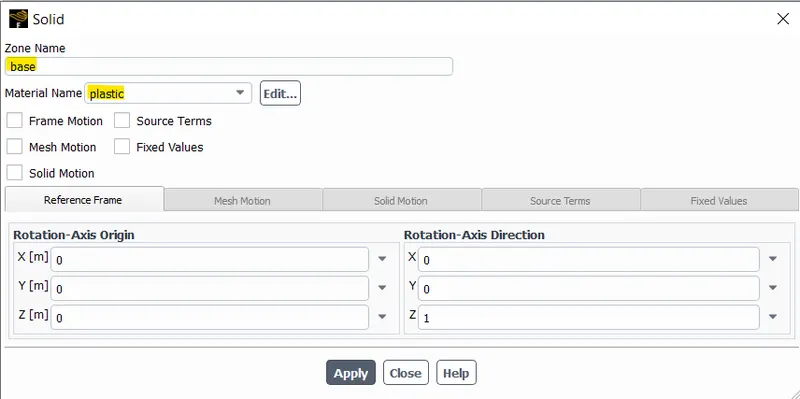
The processor is given a source term of value 15625000 `W/m^3`. The size of the processor is 0.008m X 0.008m X 0.001m. The power wattage of the processor is 1W, Hence `(1W)/(0.008mX0.008mX0.001m) = 15625000 W/m^3`, which is the source term value of the processor.

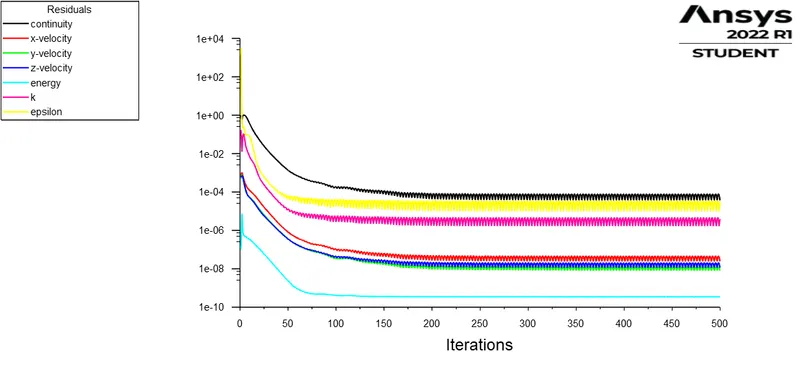
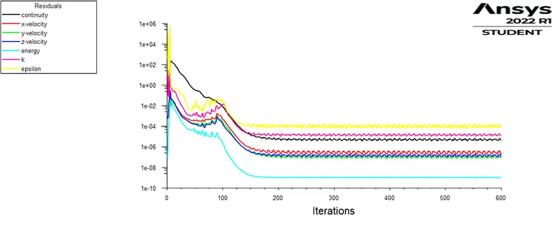
A hybrid initialization is done, with energy residual added and the convergence criteria is set to 1e-6 and the solution is calculated.

Results:

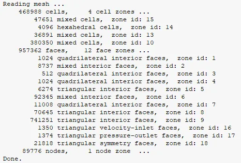
Mesh data:

Plots:

Case 1: Velocity=1m/s	Case 2: Velocity=3m/s	Case 3: Velocity=5m/s
Residuals:	Residuals:	Residuals:
Temperature plot:	Temperature plot:	Temperature plot:
Velocity plot:	Velocity plot:	Velocity plot:
Wall heat flux:	Wall heat flux:	Wall heat flux:
Temperature plot:	Temperature plot:	Temperature plot:
Total temperature in fins:	Total temperature in fins:	Total temperature in fins:
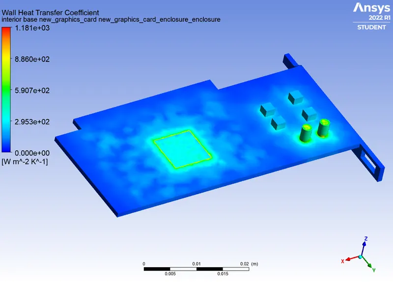
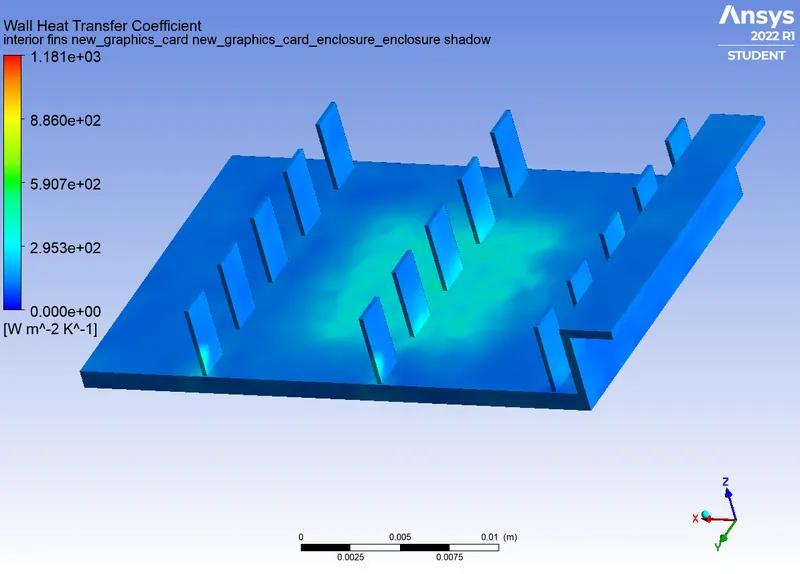
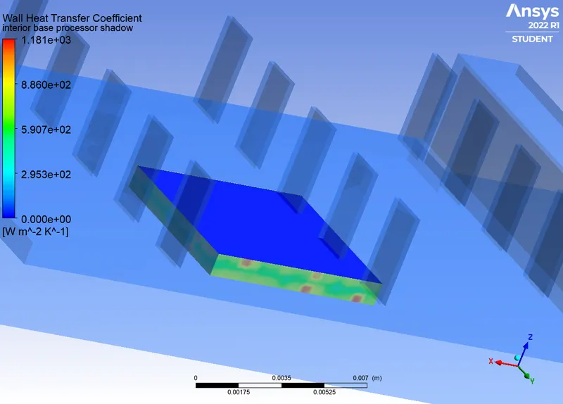
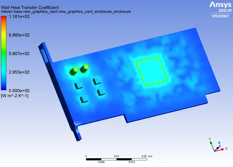
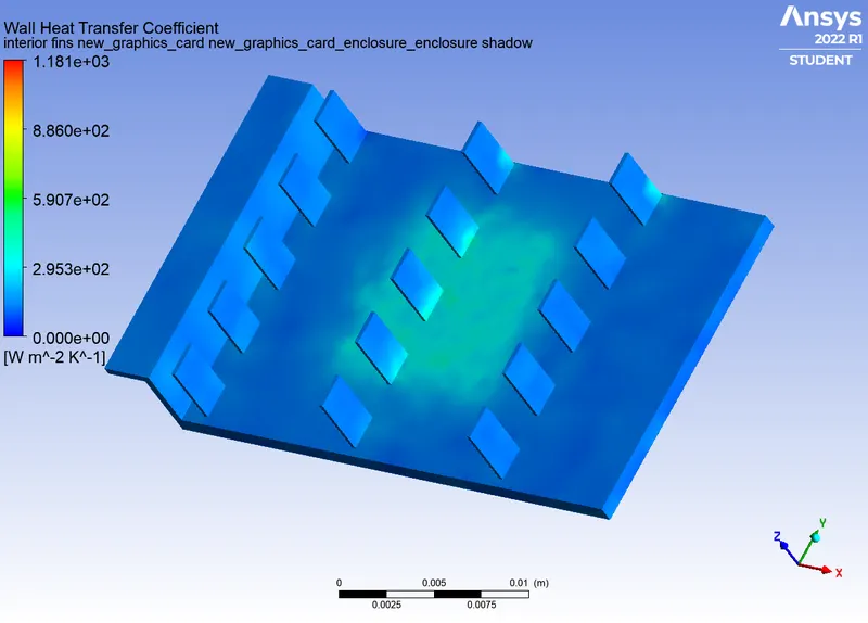
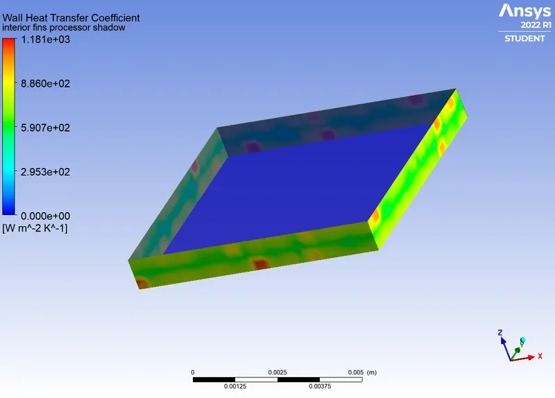
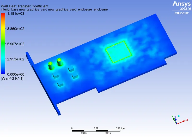
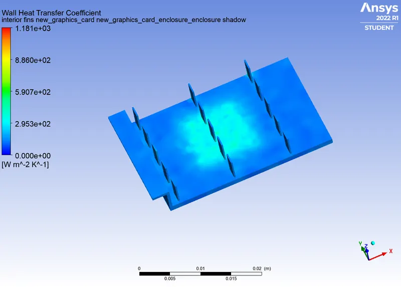
Wall heat transfer coefficient:	Wall heat transfer coefficient:	Wall heat transfer coefficient:

Computed values:

	Case 1: 1m/s	Case 2: 3m/s	Case 3: 5m/s
Total heat transfer rate	1.0000003 W	0.9999994 W	1.0000007W
Average wall heat transfer coefficient	590.7 `W/(m^2.K)`	590.7 `W/(m^2.K)`	590.7 `W/(m^2.K)`
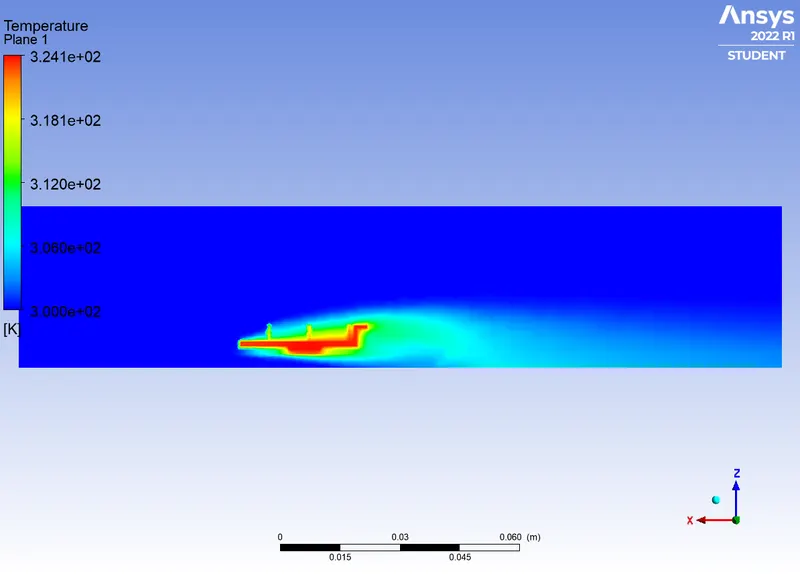
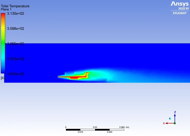
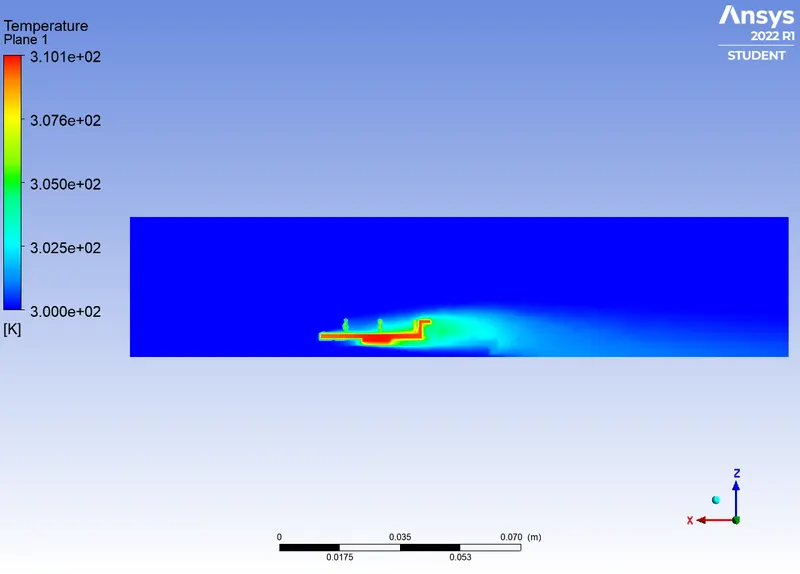
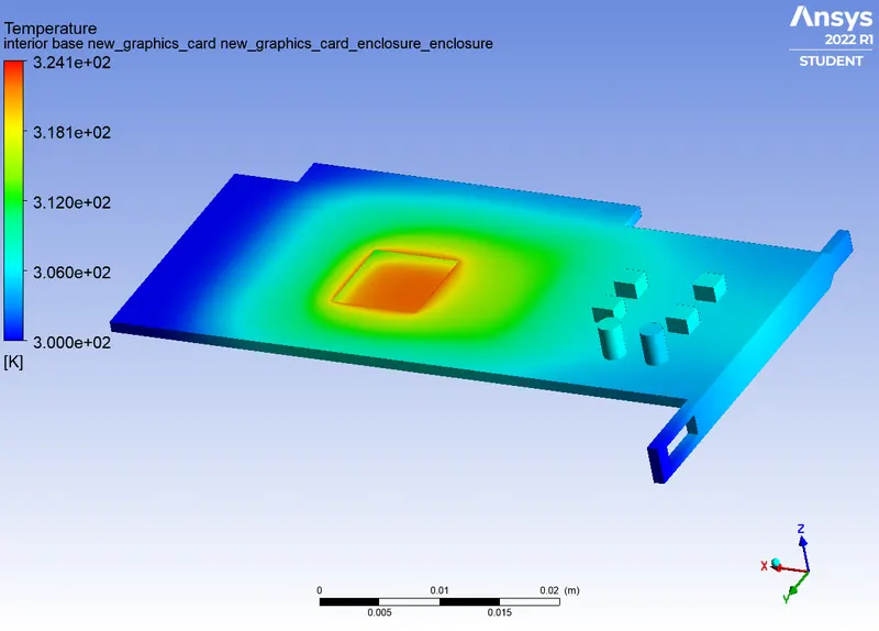
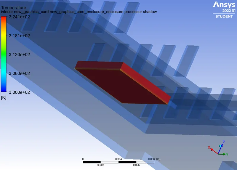
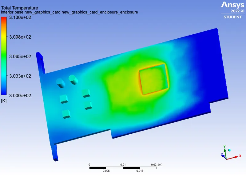
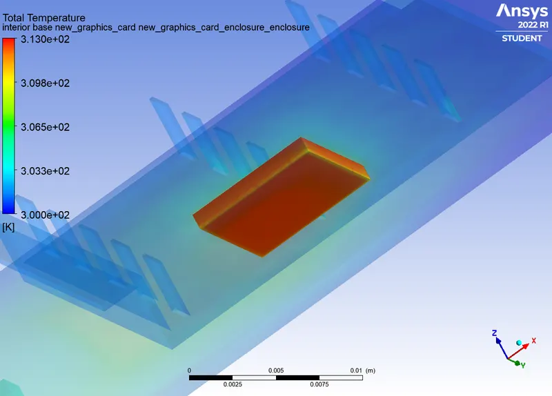
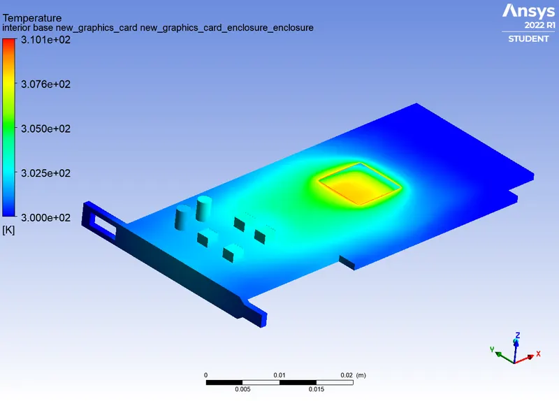
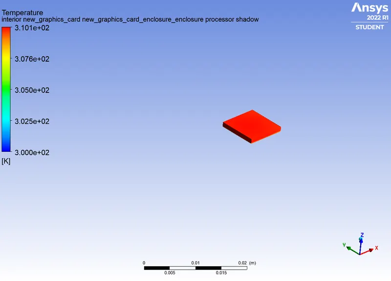
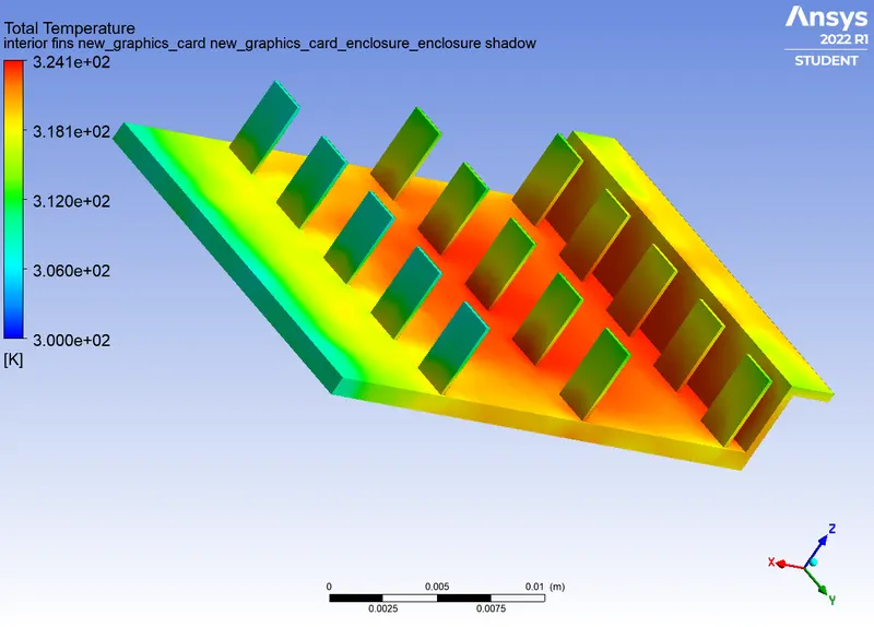
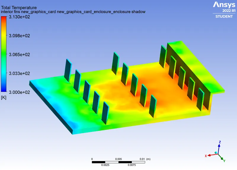
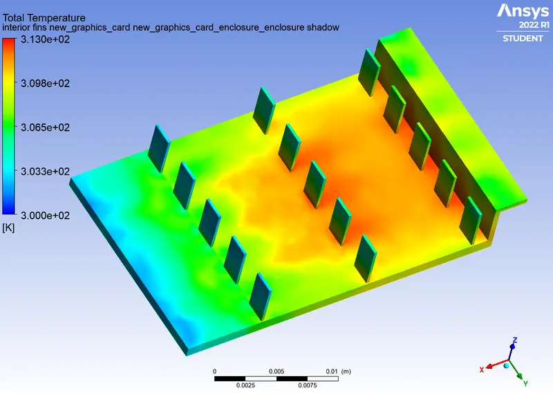
Maximum temperature	324.1 K	313.0 W	310.10 W

Inference:

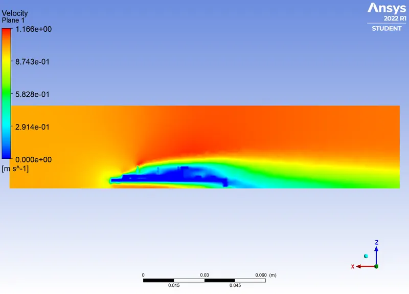
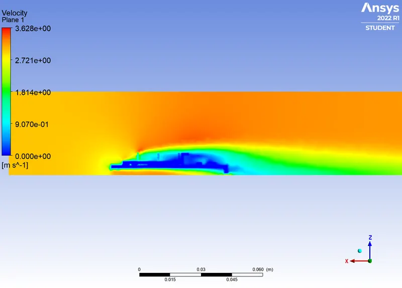
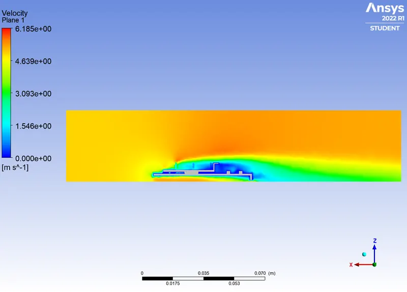
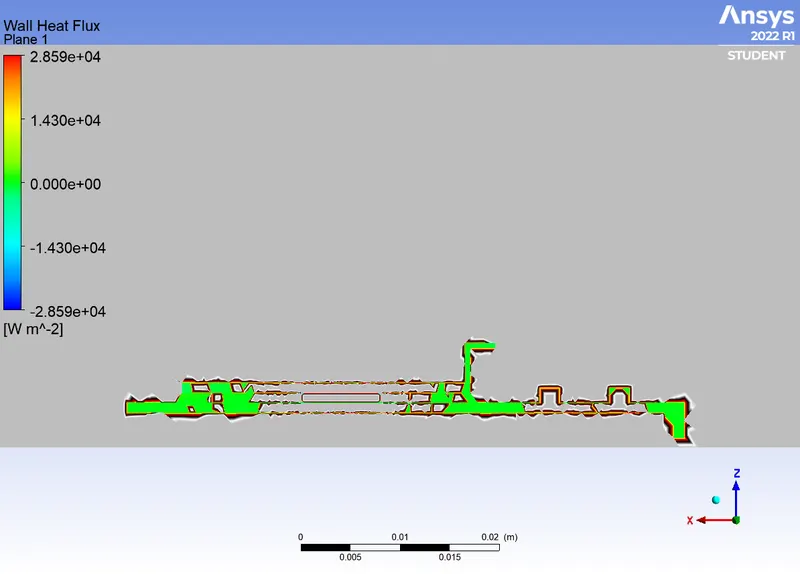
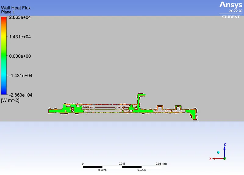
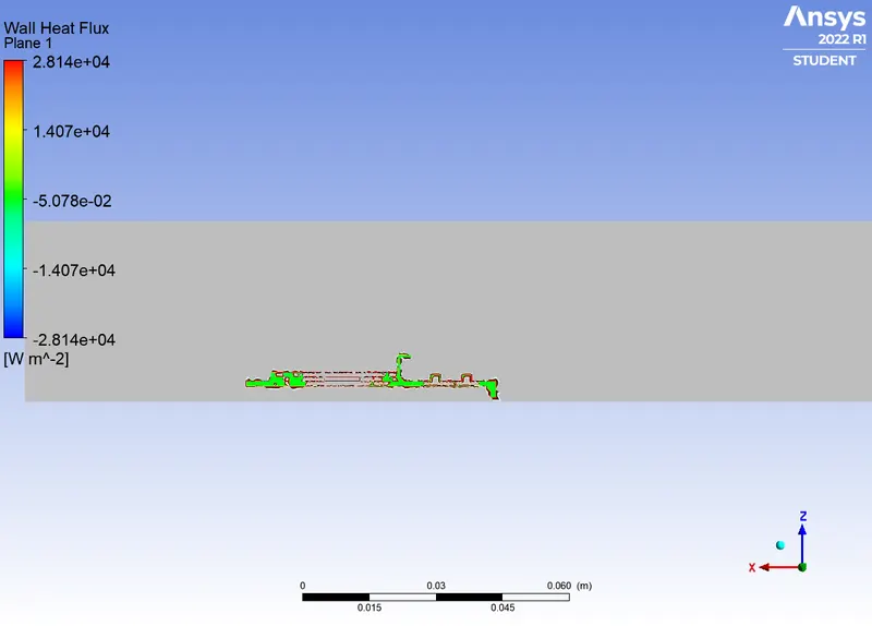
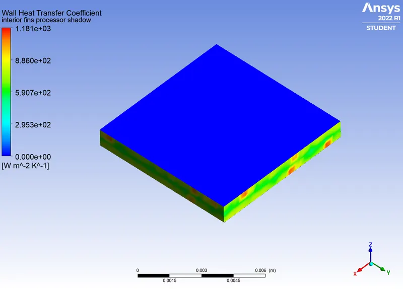
From the results, it is evident that the heat transfer rate is equal to 1W, which is the source from the processor. From the velocity plot, lower velocity fluid flow gets disturbed. A higher velocity flow is not easily diverted and hence temperature distribution rate is more even. The temperature plot says that, the temperature of the components seem to disperse with the fluid. More the velocity of the fluid, less the less spreads within the area but the discharge of the heat to the fluid environment is more. A higher velocity flow is seen to have higher heat distribution by the usage of fins. The total temperature plot is evident for the fact that a higher velocity flow is much safer for the components. The wall heat flux at the interfaces of the solid and fluid interface is seen by the shadow layer formation. There is a higher flux at the point of contact of fluid with the solid and a lower flux at the edge surfaces of the components. The wall heat transfer coefficient is more near the processor proximity and so the components at the base have higher coefficients. The side walls of the processor has higher coefficients due to the fluid motion above the surface.

Hotspots in the Graphic card:

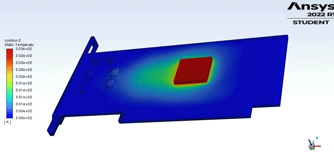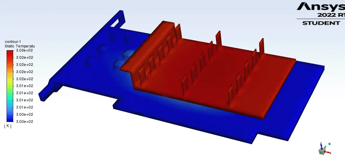
The animations show that the processor is operating in a steady state, though the temperature of the processor is high, it is cooled by fins places above it. other components near the processor seems to be in the heat proximity of the processor and hence need to be material refined. In modern day technologies liquid cooling is used which is a application of a fluid in the surfaces of the circuit and its necessity is predicted in this simulation model.

Meshing scenario:

The conformal mesh is checked in accordance with the shared topology method. The processor with fins, base and enclosure is shown below.

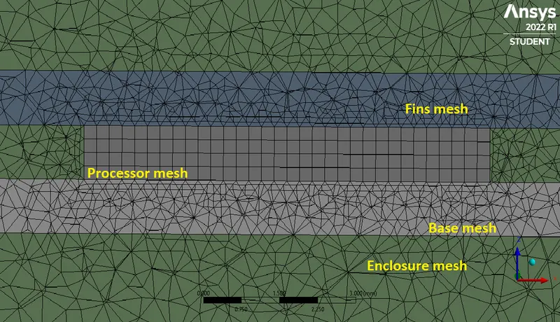
The processor is given a higher refinement as it is the power source with a smaller surface area. The element size is maintained very small in comparison to the other components, as the aim of the simulation is to identify the processor durability, keeping in mind the total number of cells executable in the academic version. The components of the base is also given a body sizing as these components would also be included in the durability calculation. The fins are given a body sizing to add accuracy to the simulation.

Convergence scenario:

Convergence criteria 0.001

Convergence criteria 1e-6

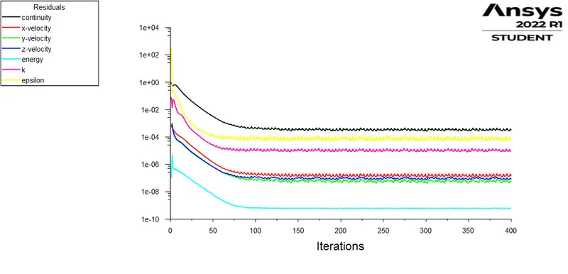
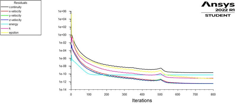
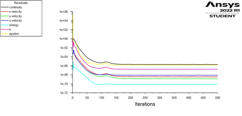
From the residuals plot, it is evident that the solution has converged. The initial convergence criteria was set as 0.001, in which case the solution was observed to get converged at about 180 iterations. Hence the criteria was decreased to 1e-6, and the convergence is observed at about 550 iterations. The solution animation also adds up to the evidence that the heat generated from the processor is radiated through the fins, which after the solution convergence iteration has not increased in temperature and velocity too. All these characteristics prove that the solution has converged.

Conclusion:

Thus the graphic card durability is measured from the simulation. It is further observed that the closer proximity of the processor with the other components reduces the durability. The fins and base on which the processor is mounted on has a quite convincing design. A high velocity fluid flow ensures convenient cooling of the circuit. The materials used is selected as per practical applications, and the results can be used to further get a clear idea of material properties to be used in the circuit manufacturing.