Week 6 - CHT Analysis on a Graphics card
AIM:
To perform a steady-state Cojugate Heat Transfer analysis on a model of graphic card with proper materials selection for simulation.
To Mesh the geometry with a desirable combination and explain the mesh setting used on this model.
Simulate the model by varying the velocity from 1m/s to 5m/s for atlease three velocities and discuss the results.
And to find out the maximum temperature and heat transfer coefficient attained by the processor along with proving that the simulation has achieved convergence with appropriate images and plots.
Finally identify the potential hot spots on the model.
DESCRIPTION:
CONJUGATE HEAT TRANSFER ANALYSIS:
The CHT analysis type allows for the simulation of heat transfer between solid and fluid domain by exchanging thermal energy at the interface between them.
In solids, conduction often dominates where as in fluids convection usually dominates.
In physics of CHT is common in many engineering applications like heat exchnagers, HVAC and electronic component design.
PROCEDURE FOR SIMULATION:
1.Import the graphics card model in the space claim and activate for share topology.
2.Mesh the model using proper element sizing
3.Open the fluent setup and perform the steady state CHT simulation on the meshed model.
4.To run the simulation for desied number or iterations so that the result get coverged and to discuss the plots.
5.Check the mesh independence of the model by performing the same simulation with different densities of mesh.
6.And to run simulation for different cases with different velocities ranging from 1m/s to 5m/s.
7.Find the maximum temperature and heat transfer coefficient attained by the processor.
8.Identify the potential hotspots on the model after the simulation.
GEOMETRY:
The geometry file is opened using Ansys work bench and it includes the model of a graphic card containing base (circuit board), processor, fins base, enclosure and other components.
The geometry and flow domain consists of a flat circuit board with heat generating electronic processor chip and some other components connected to it. Heat is conducted through the source i.e processor, the is board mounted on it and fins are attached to for heat regulation. A stream of air flows over the fins, processor and the board causing simultaneous cooling of the components and heating of the air stream due to convection. Thermal energy is also transported due to complex flow field.
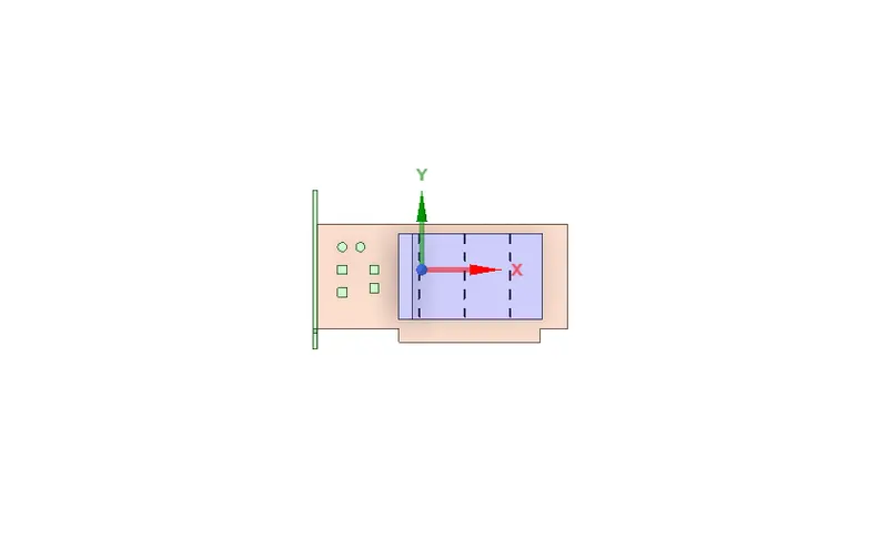
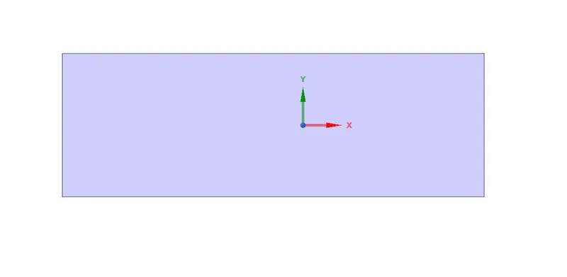
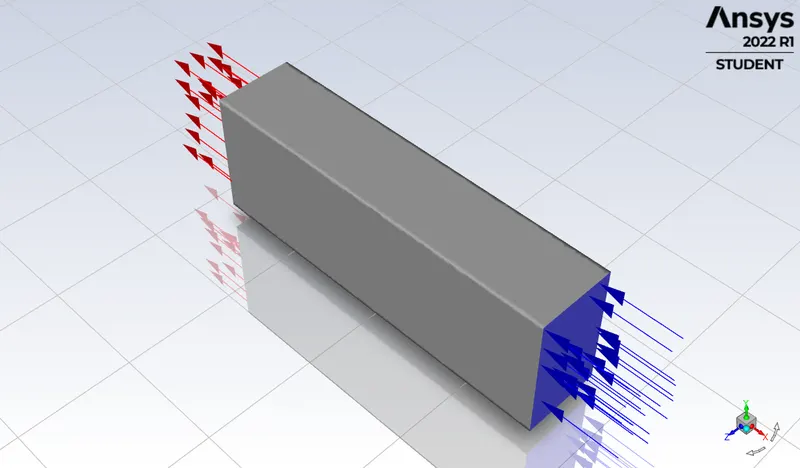
It is setup in an enclosure in which through inlet the air passes and through outlet the thermal hot air escapes in x-direction.
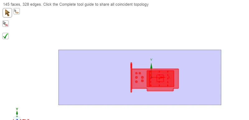
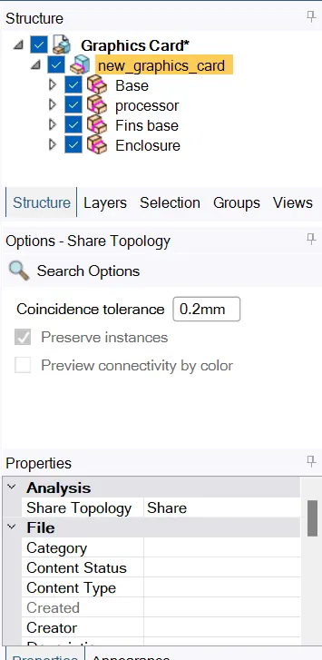
Then in the workbench selecting the share tool to get the conformal mesh so that heat is transferred in a systematic way between the cells from one component attached to another.
MESHING:
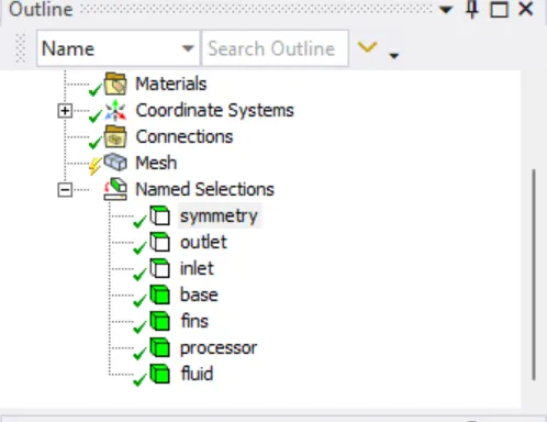
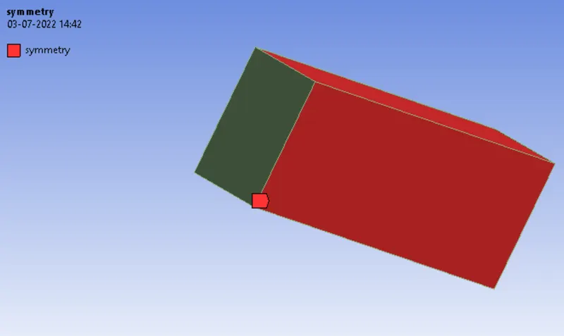
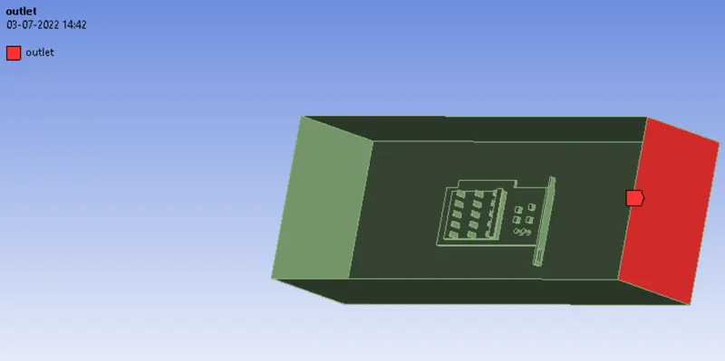
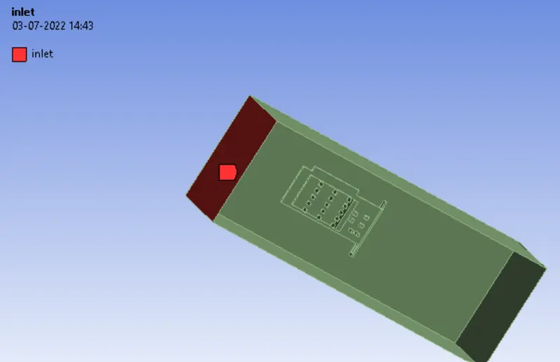
Here in meshing the first thing we do is start naming the components as follows
For symmetry
For outlet
For inlet
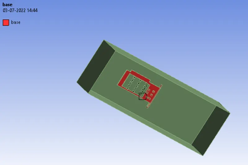
For base
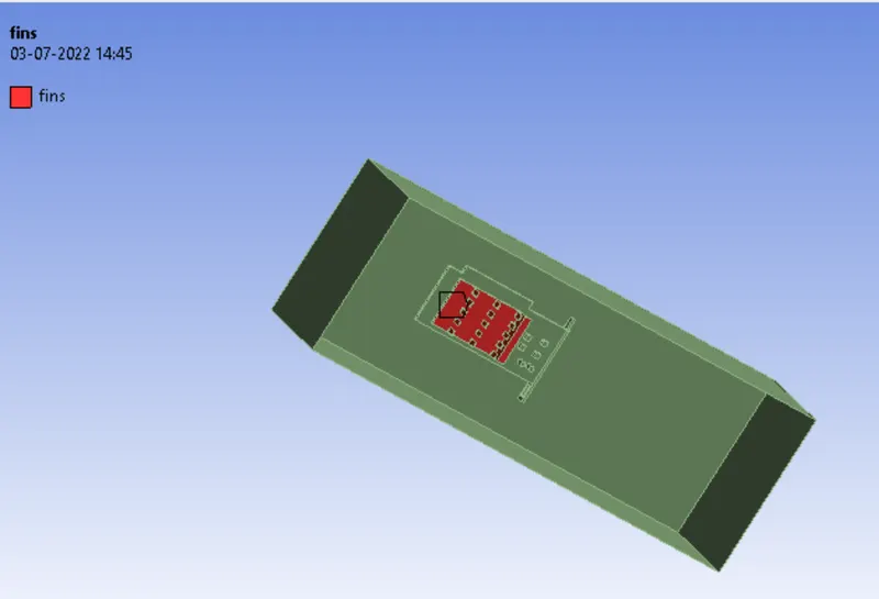
For Fins
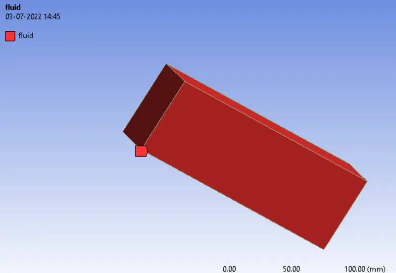
For fluid flow
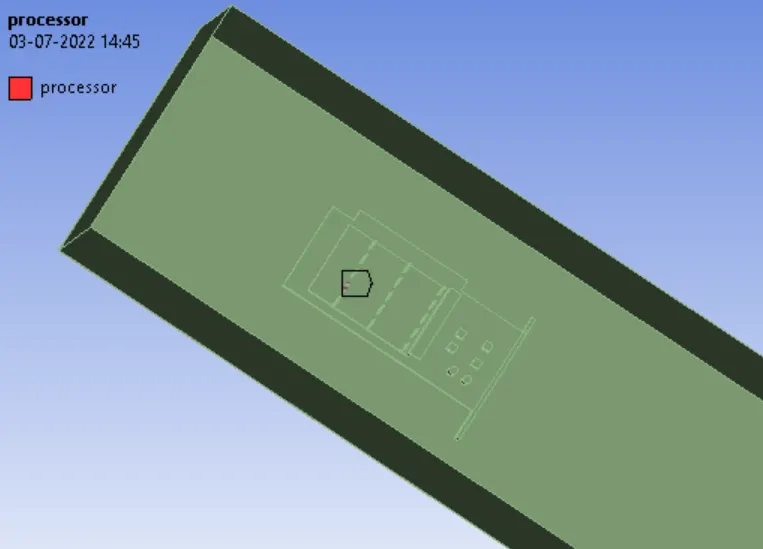
For processor
Generating a baseline mesh we get as follows
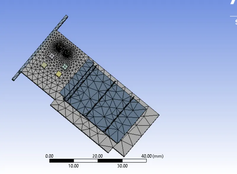
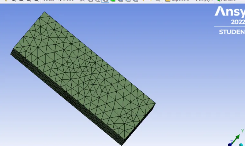
As we can see that the mesh we got is conformal with default elemental size.
ANSYS FLUENT
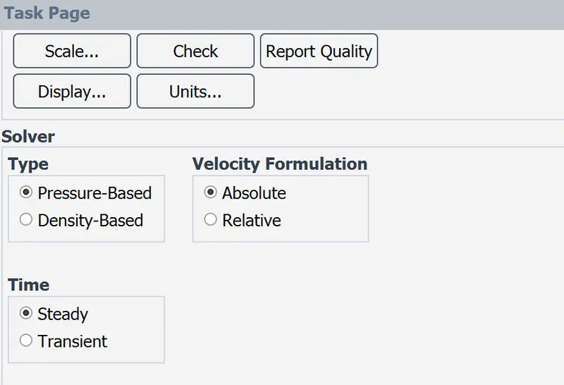
Using pressure based, steady state solver
As the temperature is being calculated for the simulation model we enable the energy equation
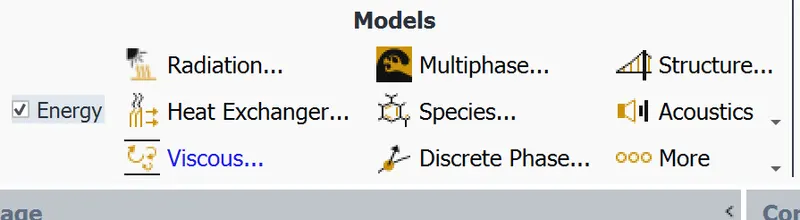
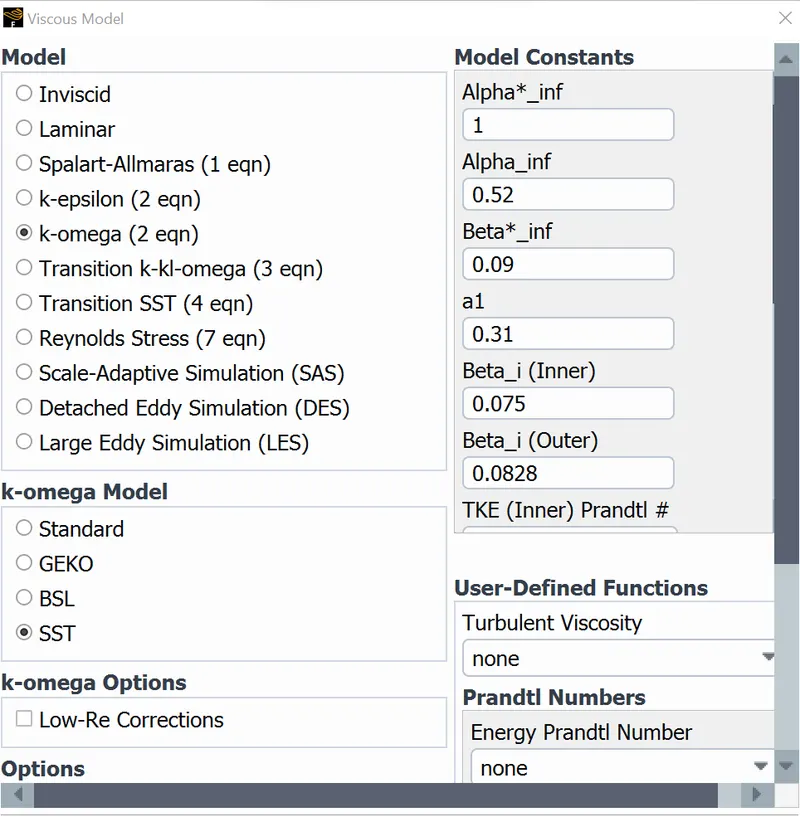
For this simulation, the k-omega turbulent model is considered which is best used for near-wall treatment.This is vital for this simulation as we expect the heat transfer coefficient on the surfaces.
For the k-omega SST model , SST is selected as it provides a better prediction of flow separation that most RANS models and also accounts for its good behaviour in adverse pressure gradients.It has the ability to account for the transport of the principal shear stress in adverse pressure gradient boundary layers. It is the most commonly used model in the industry given its high accuracy to expense ratio.
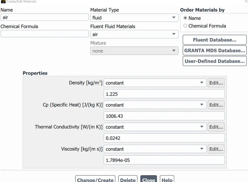
For the material selections
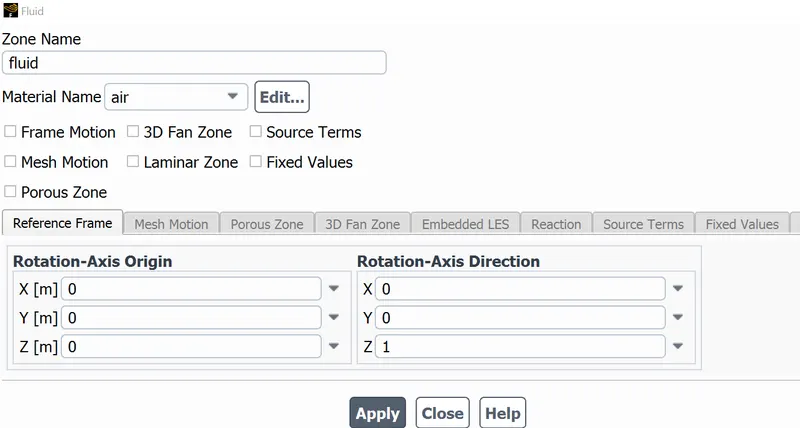
As for coolant air is used in the fluid domain
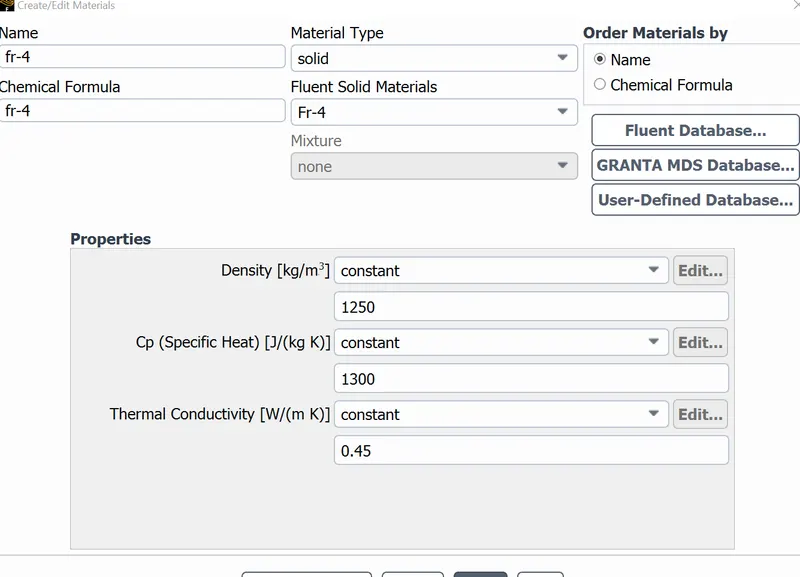
Then we use Fr-4 is a glass reinforced epoxy resin laminate that stands for Flame retardant.It has a high working temperature, good heat resistance, good moisture resistance, good hole metalization performance.Therefore, it is preferred to build PCB.
As the base plate is considered as a circuit board so FR-4 is used for it.
As this material is not present in fluent we created using fluent data base by changing the name
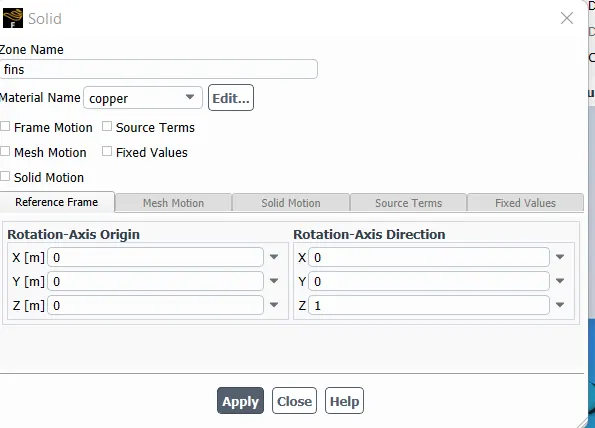
For Fins, then a copper material is taken as it is a good conductor of heat
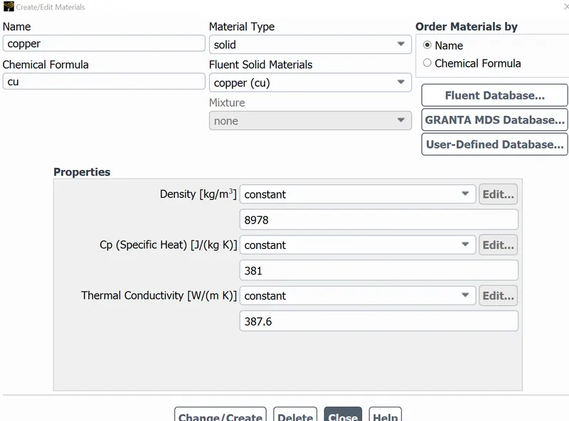
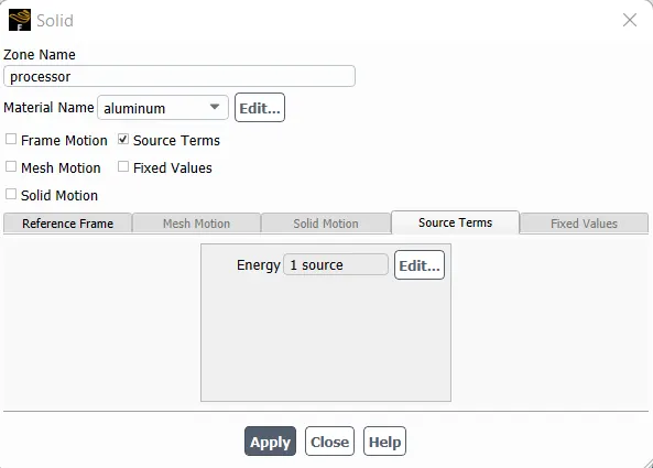
For base and other components aluminium is taken
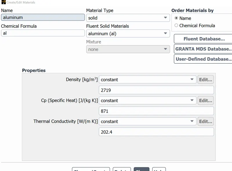
Then the cell zones materials are checked and matched as follows
For base
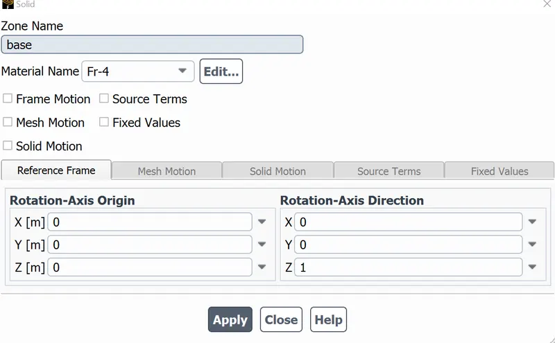
For fins
For processor
For fluid
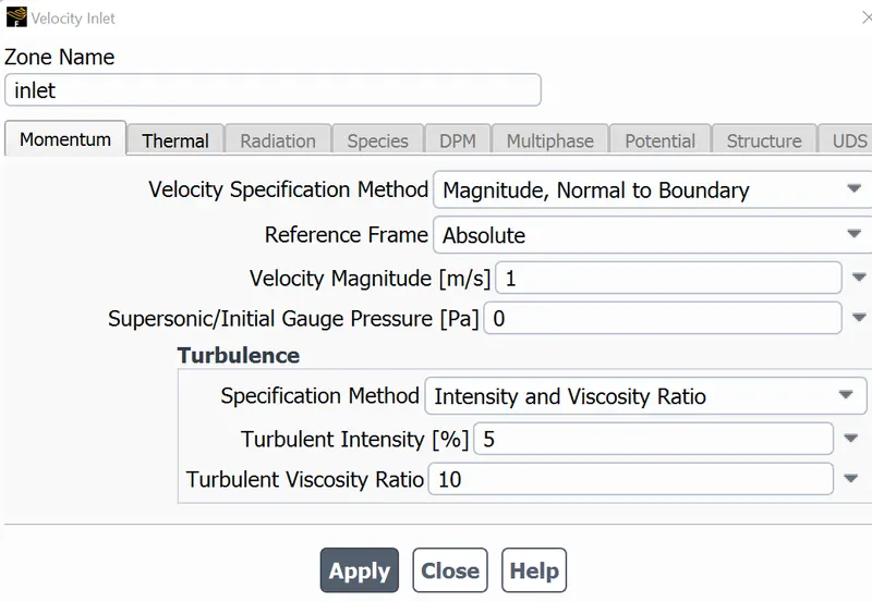
Then setting up the boundary conditions
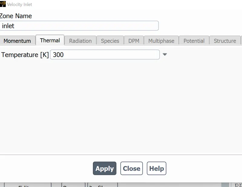
For inlet
Then calculating the processor area
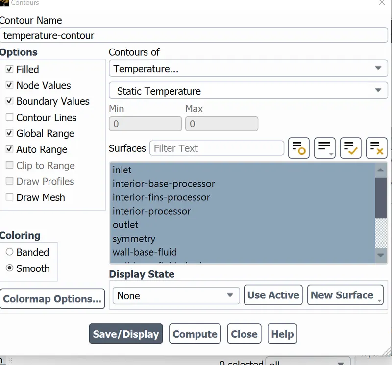
Then creating the contours
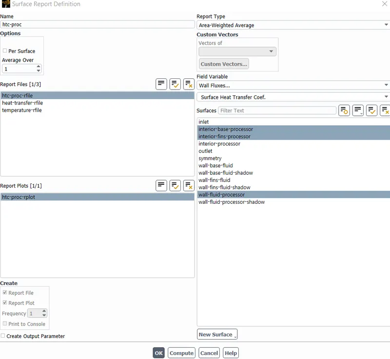
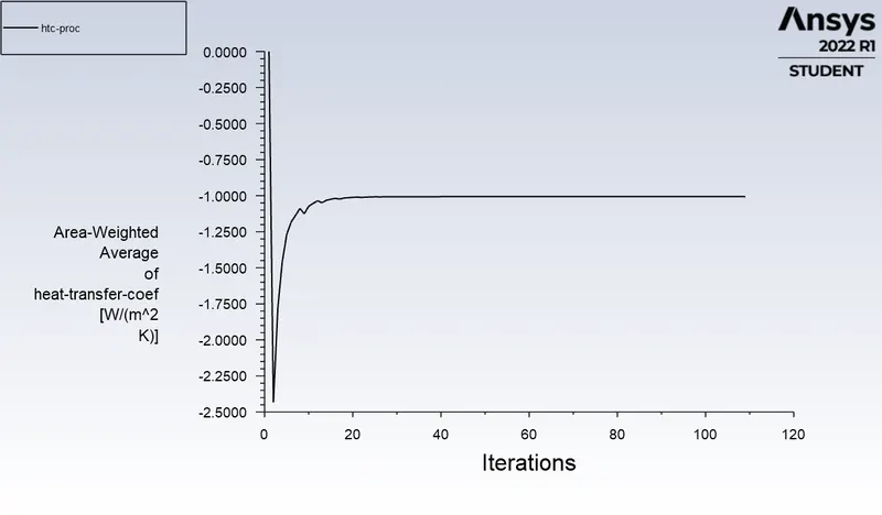
Plotting Heat transfer coefficient
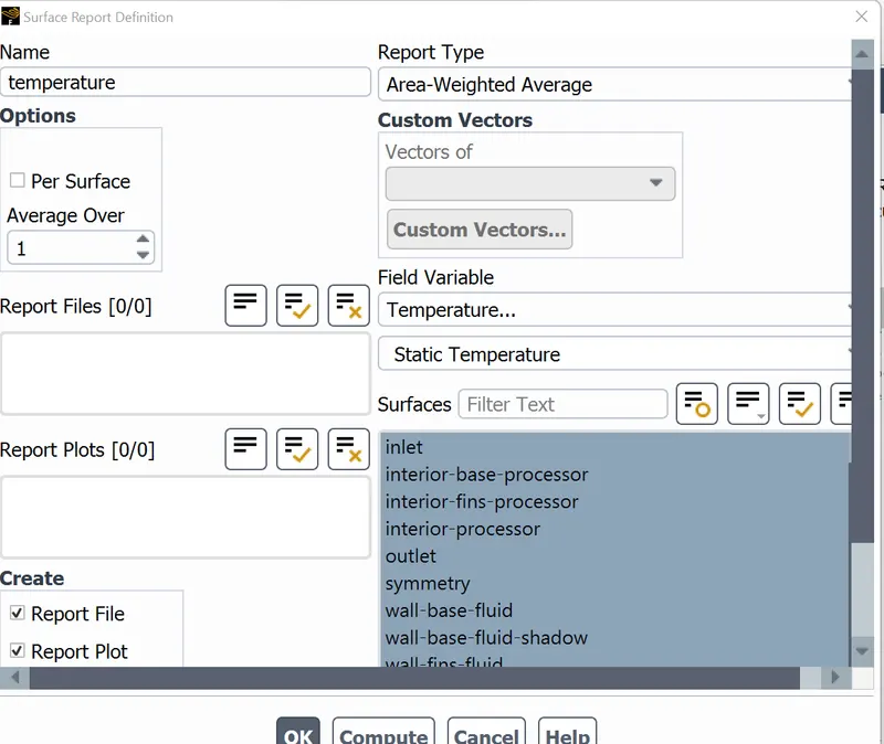
Creating the temperature graph
Giving the energy, lets assume a case of R350 GPU running at 400MHz on a 0.15micron process at 1.75v with 51.75W output where GPU run with the efficieny between 66 - 75% rest of energy is wasted in the form of heat which is 12.9375W
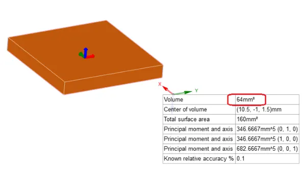
Calculating the energy, Energy = 12.9375/64e-9 = 202148437.5W/m3
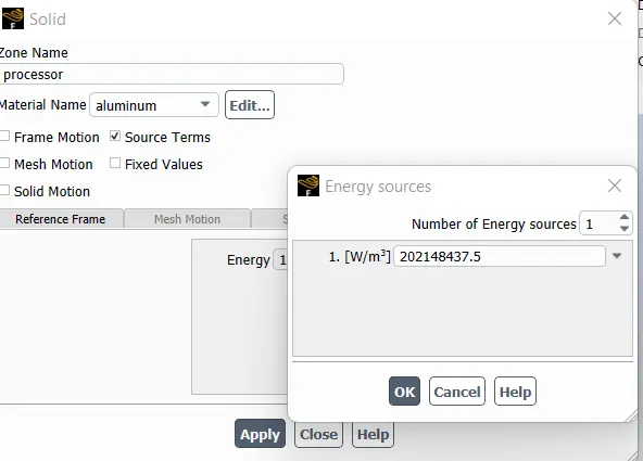
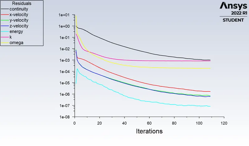
CASE-I:SIMULATION WITH DEFAULT MESH FOR 1m/s VELOCITY OF AIR FLOW
The residuals are
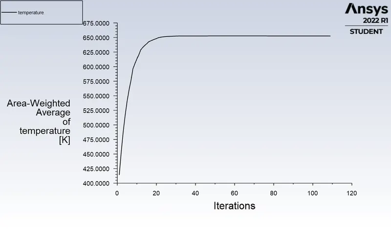
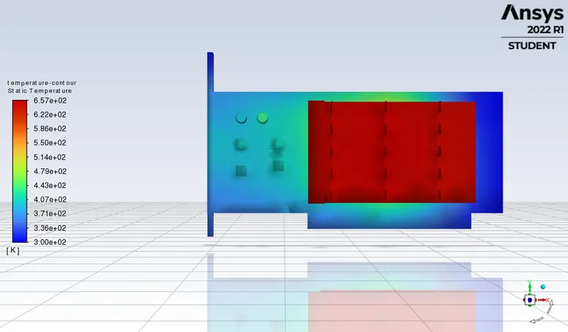
The temperatures is
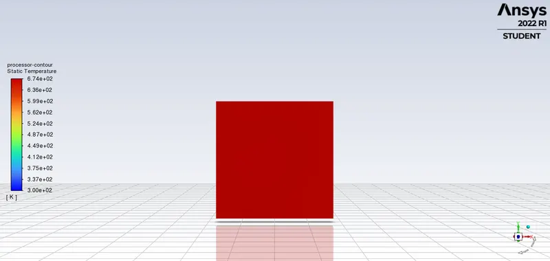
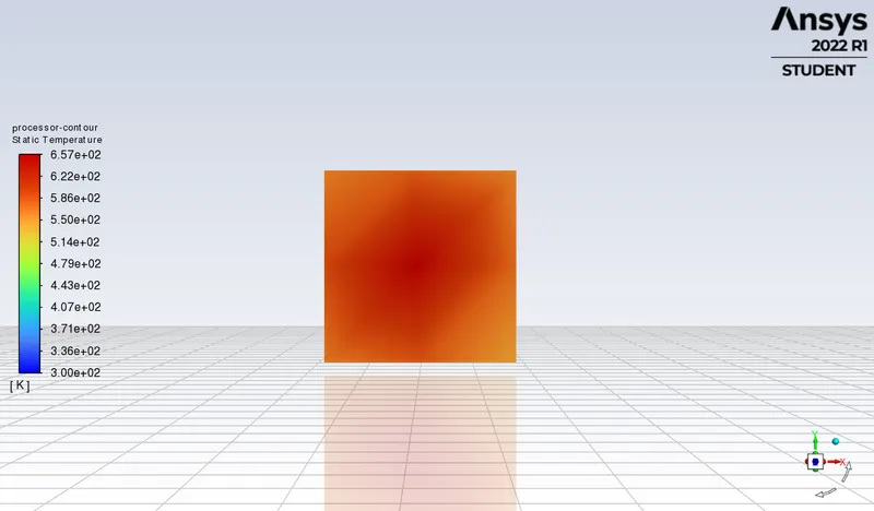
The processor contour is
The HTC is
The base contour is
htc-proc -1.0055039
temperature 652.50235
CASE-II
Changing the mesh size to 1.8mm
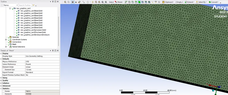
Running the simulations for 600 seconds
1.SIMULATION WITH DEFAULT MESH FOR 1m/s VELOCITY OF AIR FLOW
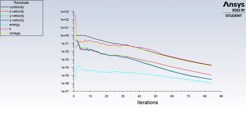
The residual plots are
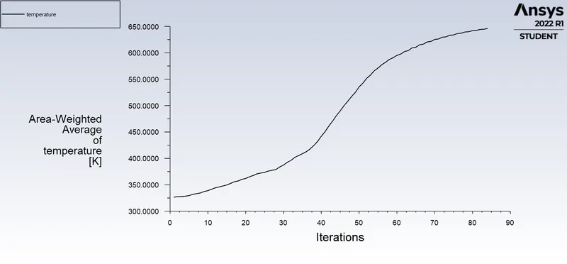
The temperature plots are
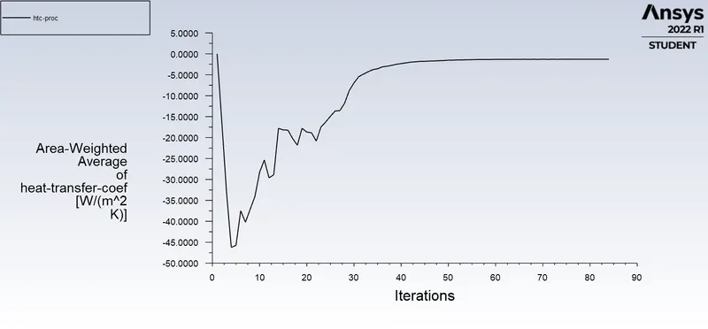
The HTC is
The base contour is
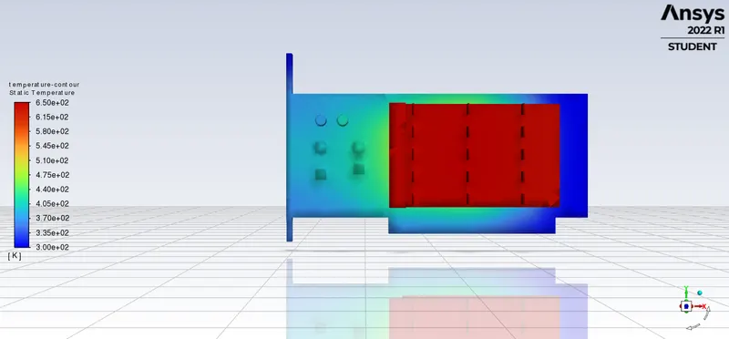
The processor contour is
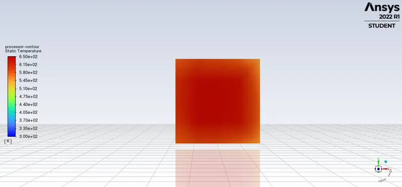
The base contour is
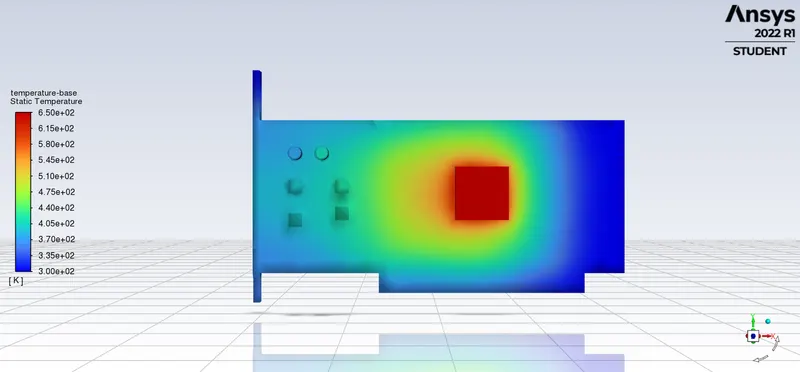
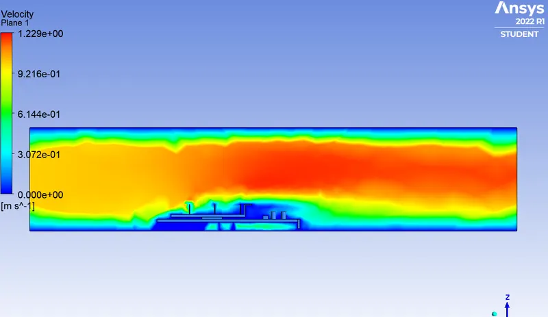
The velocity plane is
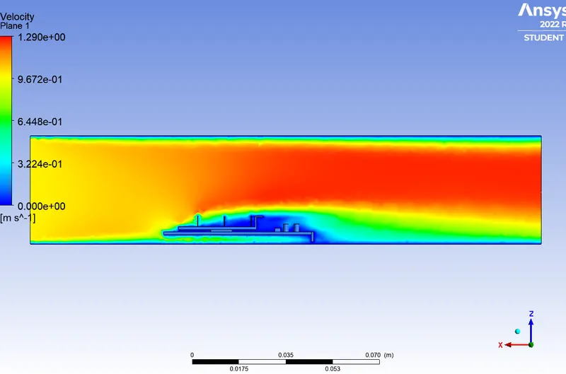
temperature 646.1916
htc-proc -1.2835967
2.SIMULATION WITH DEFAULT MESH FOR 2m/s VELOCITY OF AIR FLOW
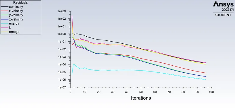
The residual plots are
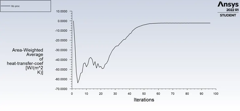
The HTC is
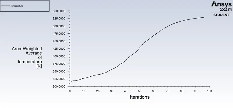
The temperature is
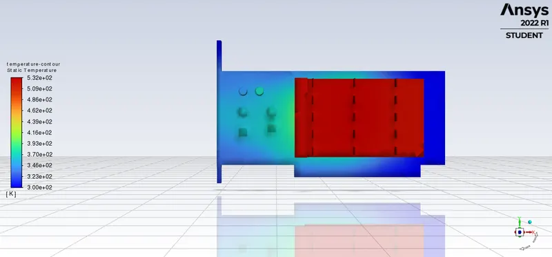
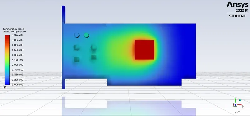
The base contour is
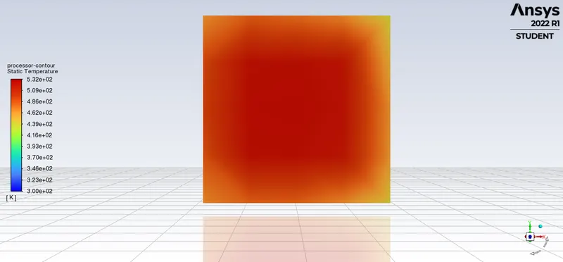
The processor contour is
The velocity flow plane is
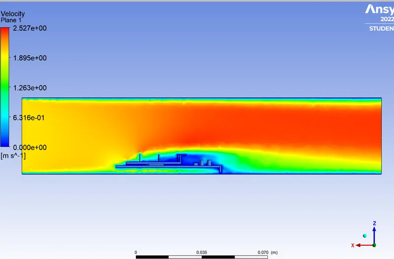
temperature 528.36377
htc-proc -2.2926717
3.SIMULATION WITH DEFAULT MESH FOR 3m/s VELOCITY OF AIR FLOW
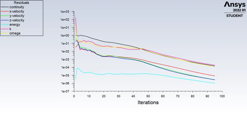
The residuals are
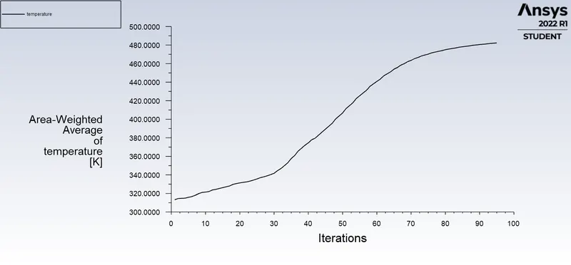
The temperature is
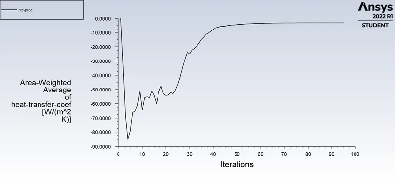
The HTC is
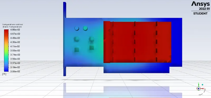
The base contour is
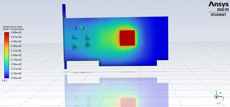
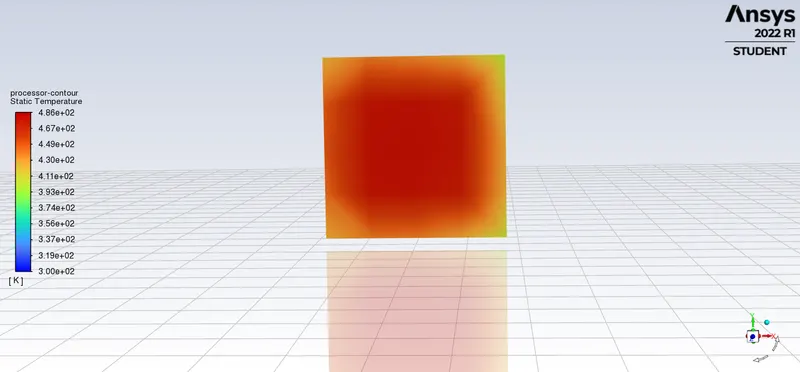
The processor contour is
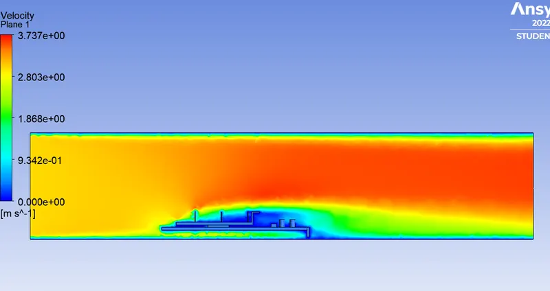
The velocity flow plane is
htc-proc -3.1513713
temperature 482.29117
4.SIMULATION WITH DEFAULT MESH FOR 4m/s VELOCITY OF AIR FLOW
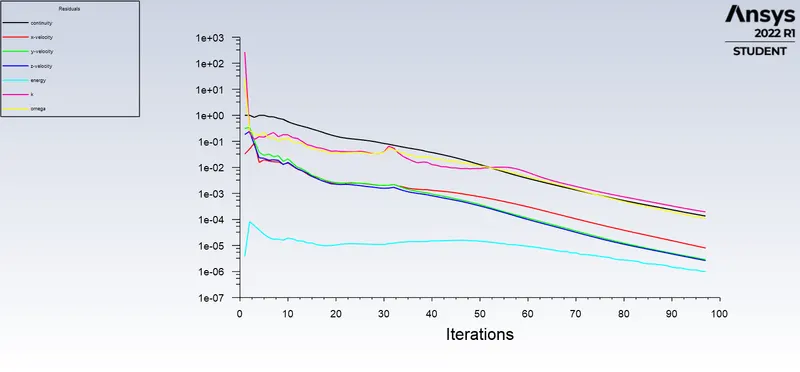
The residuals are
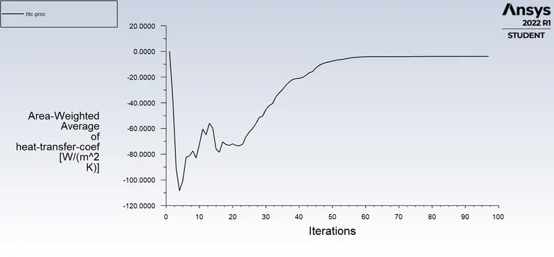
The HTC is
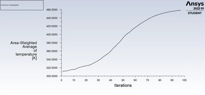
The temperature is
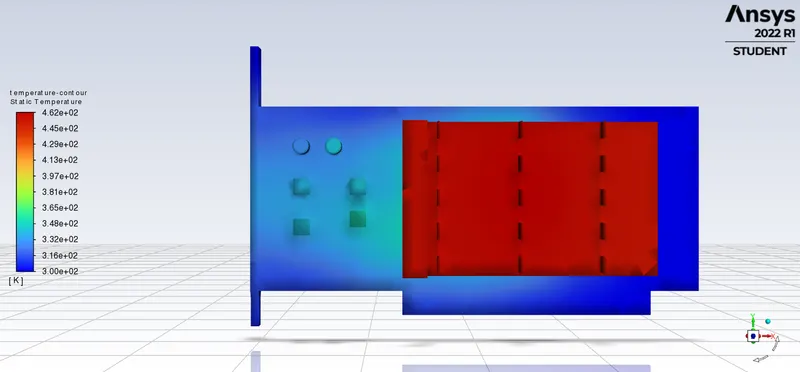
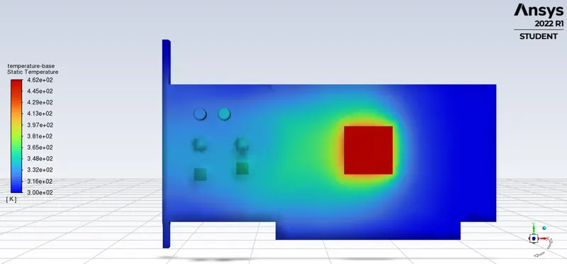
The base contour is
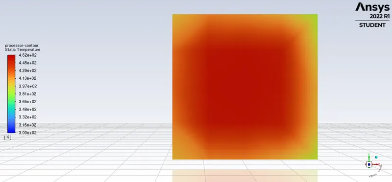
The processor contour is
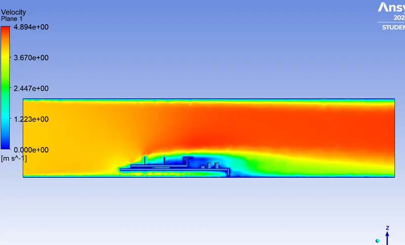
The velocity flow plane is
temperature 458.28873
htc-proc -3.8499011
RESULTS:
The initial temperature was 300K
| TEMPERATURE(K) | HTC (W/m2K) | |
| CASE-I velocity 1m/s |
646.1916 |
-1.2835967 |
| CASE-II velocity 2m/s | 528.36377 | -2.2926717 |
| CASE-III velocity 3m/s | 482.29117 | -3.1513713 |
| CASE-IV velocity 4m/s | 458.28873 | -3.8499011 |
Therefore, we see that with increase in velocity of air the temperature is gradually reducing and heat is getting regulated in a good manner and even heat transfer rate per unit area is gettinng regulated properly.
IDENTIFYING POTENTIAL HOTSPOTS ON THE MODEL:
The potential hotspots on the model are the processor which generates the heat and to which is attached the fins for heat regulation and the fins which are made up of copper which shows that the heat transfer is in a well regulated manner as its made of copper which is a very good conductor.
CONCLUSION:
Higher velocity means higher Reynolds number so that is the reason heat transfer coefficient is highest at that area, which means the maximum amount of heat transfer is taking place from fluid to solid in the model.This also results in a higher temperature of solid in that model.
Heat transfer coefficient is a function of properties of the fluid at film temperature, temerature difference, temperature coefficient, buoyance force etc hence mesh resolution near walls ususlly has the biggest impact on numerical results.
For the turbulent models we have to take care of the assumptions and the boundary conditions you put in the program.The mesh is a very important parameter to get nice results so we have to refine it in the important place of our drawing.
Some factors should be considered which is the most significant in the turbulent boundary layer, if we are using any kind of low Reynolds turbulence model considering enhanced wall treatment. so we need to make sure that we stay in the laminar sub-layer region where the velocity profiles are assumed to be laminar and viscous stress dominates the wall shear.
The mesh/grid dependency test is very important to get the over all results verified.