Week 6 - CHT Analysis on a Graphics card

CHT Analysis on a Graphics card

Aim:Is to Perform a steady-state conjugate heat transfer analysis on a model of a graphics card. You can use appropriate materials of your choice for the simulation. Make sure to properly define the correct solid and fluid zones. Refer the video for further clarification and the model is provided below the video.

Run the simulation for best possible mesh with combination of coarse and refined mesh in different regions. Explain the reason for choosing the particular mesh settings.

our Objectives:

1. Run the simulation by varying the velocity from 1m/sec to 5m/sec for at least 3 velocities and discuss the results.
2. Find out the maximum temperature and heat transfer coefficient attained by the processor.
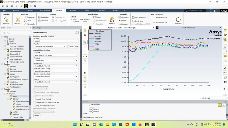
3. Prove that the simulation has achieved convergence with appropriate images and plots.
4. Identify potential hotspots on the model.

Theory:

conjugate heat transfer (CHT) analysis can accurately predict heat transfer by simultaneous solving all the relevant solid and flow field heat transfer processes, for example: conduction through solids, free and forced convection in the gases/fluids and thermal radiation.

The CHT approach has an advantage over FE thermal analyses in that wall heat transfer coefficients and their local variations on surfaces are directly calculated within the model rather than based on simplified empirical calculations. The CHT approach therefore has benefits for those applications where heat transfer is either non-uniform or difficult to calculate empirically.

where and why we use heat transfer coefficent:

1. The transport of fluid implies energy transport too, which appears in the heat equation as the convective contribution. Depending on the thermal properties on the fluid and on the flow regime, either the convective or the conductive heat transfer can dominate.
2. The viscous effects of the fluid flow produce fluid heating. This term is often neglected, nevertheless, its contribution is noticeable for fast flow in viscous fluids.
3. As soon as a fluid density is temperature-dependent, a pressure work term contributes to the heat equation. This accounts for the well-known effect that, for example, compressing air produces heat.

CHT Analysis on a Graphics card

case 1: base line stimulation

steps invalving in analysis of flao through the exhoust port:

1. Geomatry
2. meshing
3. setup
4. solution
5. result

Geometry: first step is importing the geometry in to the space claim as shown below

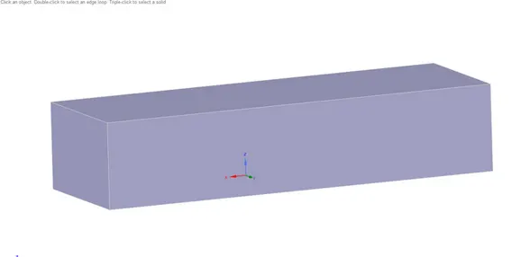
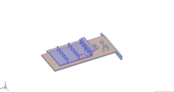
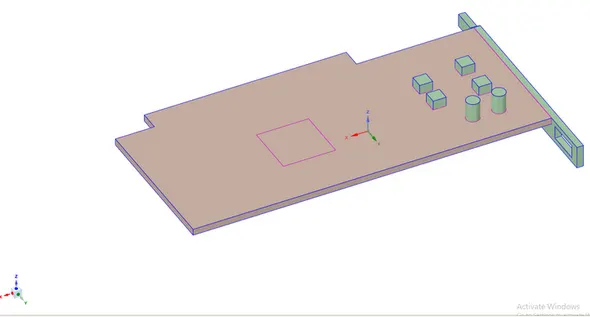
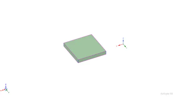
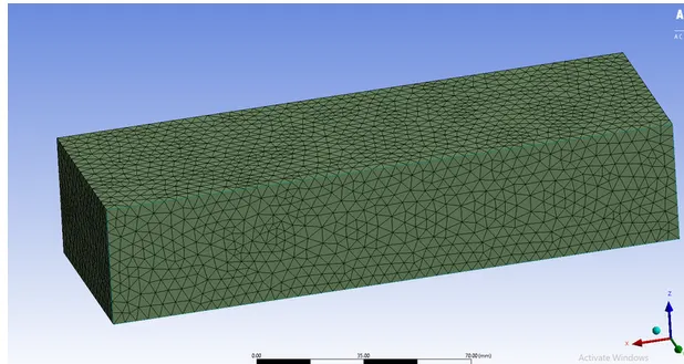
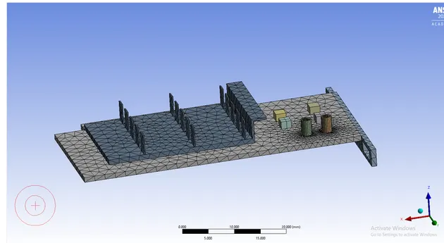
• meshing:first we have to create the base line mesh before that we have to name the parts as shown below

setup:

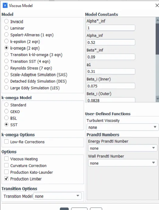
• first we have to setup the physics in physics we are using k omega as viscouse model and then we are assuming the inlet body condition as 1m/s,and tempreture as 300k as shown below

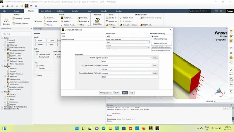
• after seting physics we have to create the material for the fallowing parts we we have taken

1. fins: it is made up of copper
2. processer: it is made up of alluminium
3. base; it is made up of steel
4. enclosure: we have air

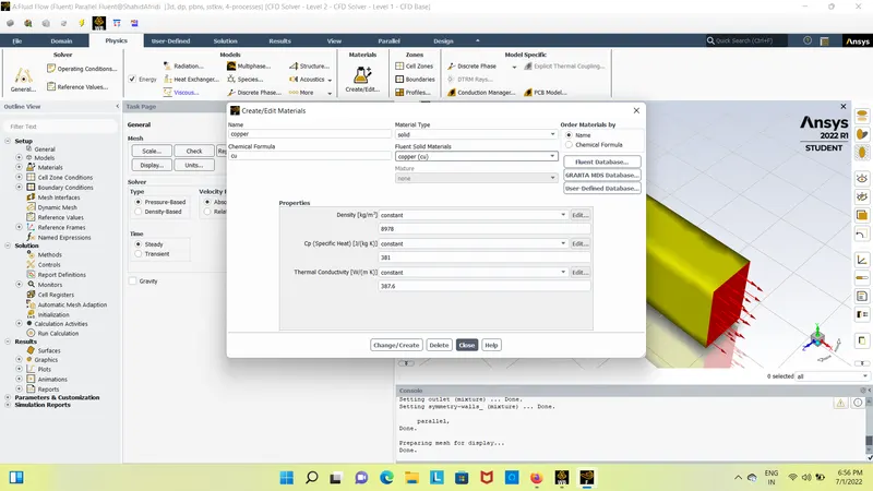
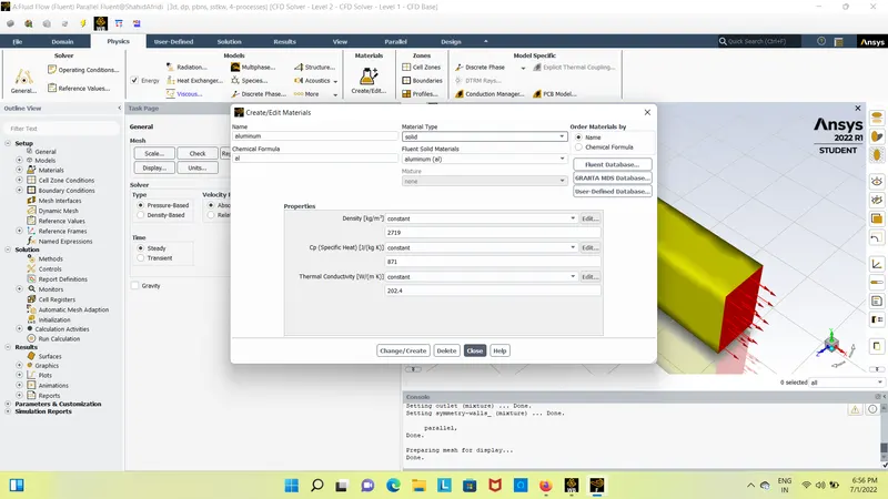
solution and results:

heat produced by processer:

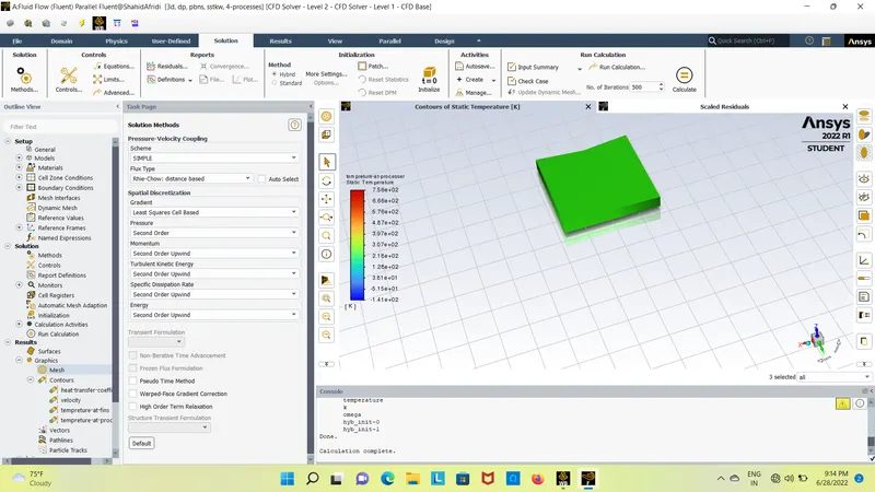
residuals:

heat transfer coefficent:

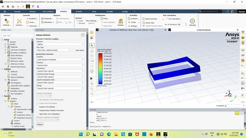
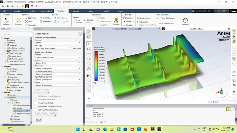
tempreture at fins:

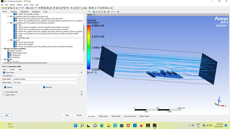
velocity steamlines:

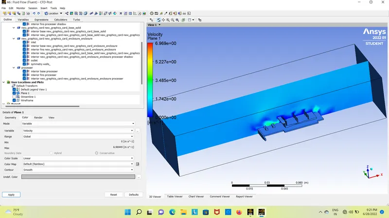
velocity plane:

case 2: refining the mesh and also for velocity 1m/s

geometry:it is same as above

meshing: here we are refining the mash as shown below

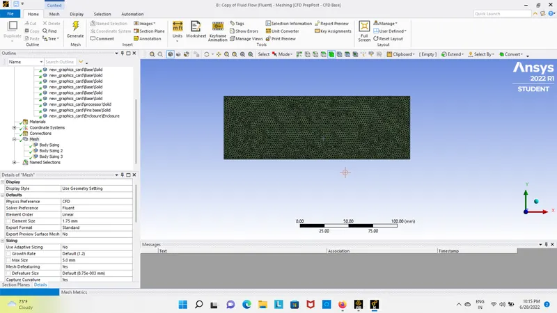
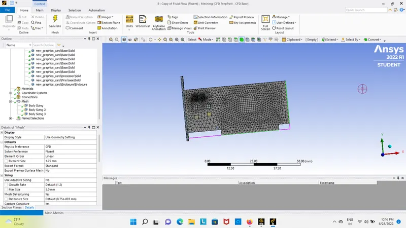
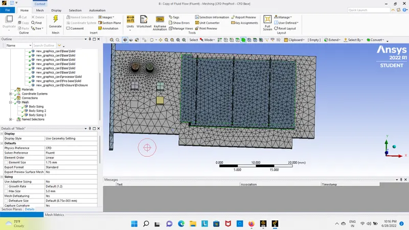
setup: as same as above

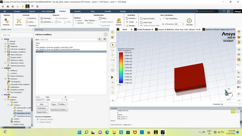
solution:here we are just changing the velocity as 3m/s

processer:

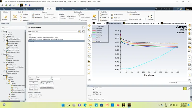
residuals:

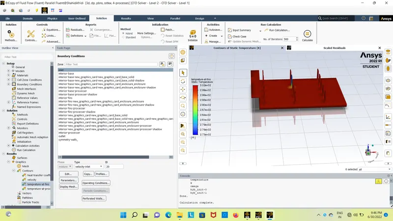
tempreture at fins:

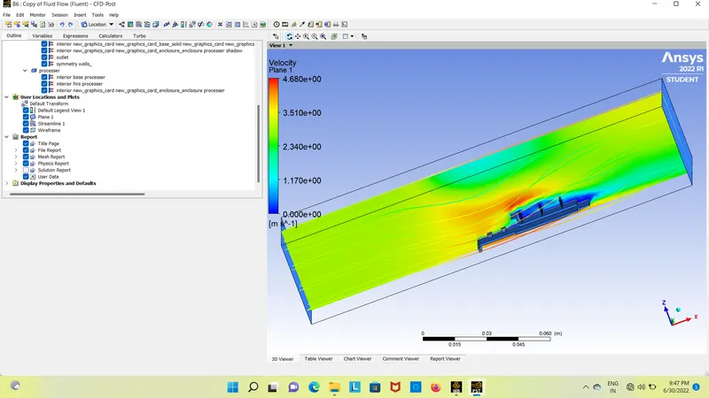
velocity plane:

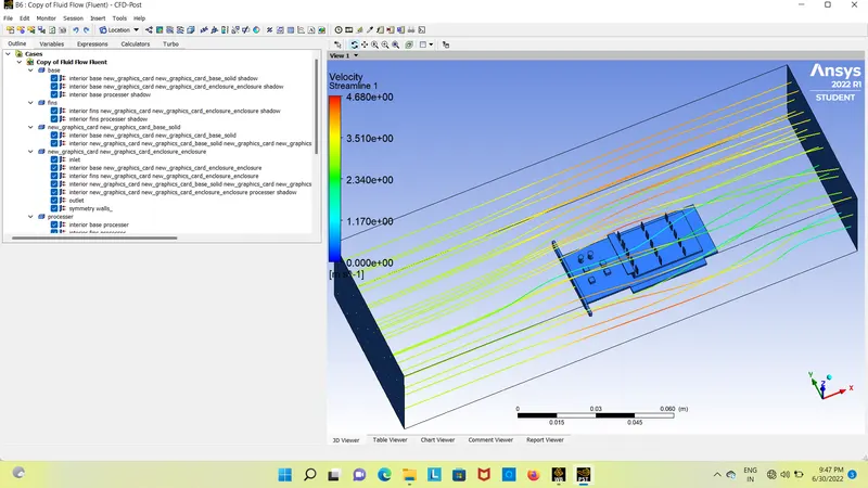
velocity steamlines:

case 3: velocity 5m/s

geometry:it is same as above

meshing: it is also same as above

setup: it is also same as above

solution:

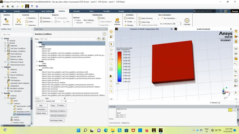
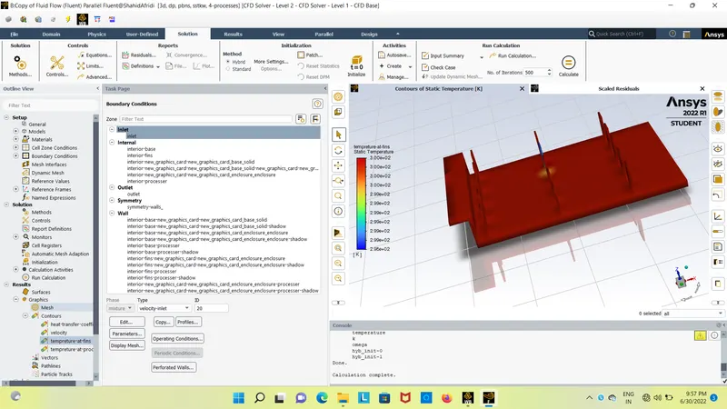
tempreture at fin:

residuals:

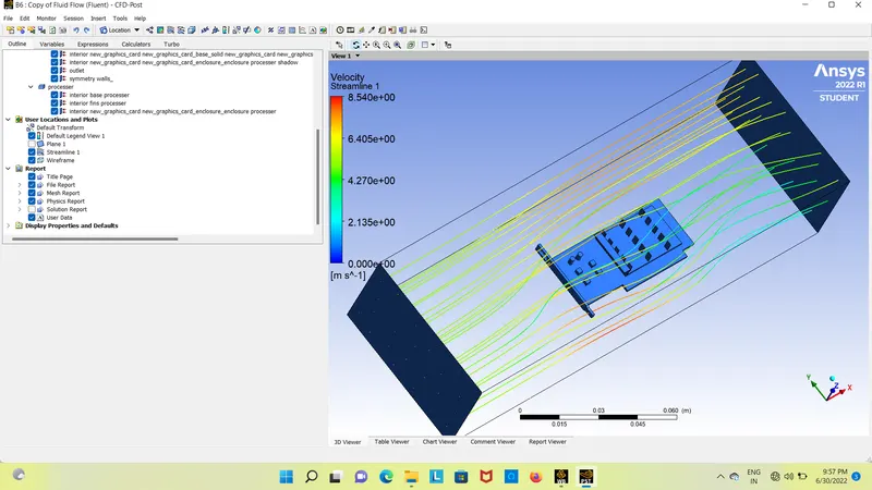
steamlines:

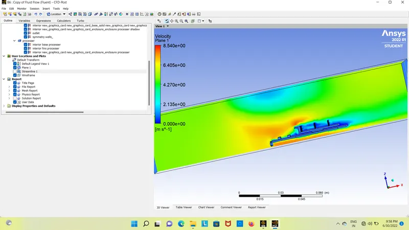
velocity plane:

Conclution: as we know processer is the one which producess heat and it is the only source of producing heat so it is the main hotspot of the given project

• the maximum tempreture attained by the proceesr is 300k
• and also we can observe that as we increse the velocity the tempreture at processer is decreasing gradually