Week 3.5 - Deriving 4th order approximation of a 2nd order derivative using Taylor Table method

Aim: Is to Derive the following 4th order approximations of the second-order derivative.

1. Central difference

2. Skewed right-sided difference

3. Skewed left-sided difference

4.After deriving these schemes, prove that your skewed schemes are fourth-order accurate

5. After that write a program in Matlab to evaluate the second-order derivative of the analytical function exp(x)*cos(x) and compare it with the 3 numerical approximations that you have derived.

6.Provide a plot that compares the absolute error between the above-mentioned schemes

7.In your own words, describe why a skewed scheme is useful? What can a skewed scheme do that a CD scheme cannot?

1) Deriving for Central diffrence :

No of Nodes : they have given `n = p+q-1`

where n is numer of nodes

p is The order of accuracy

q is order of derivative

`n = p+q-1`

n = 4+2-1

n = 5.

using this equation we can draw the diagram for central diffrence scheme and our stencil schme look like this.

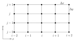
as we are solving for the 4th order approximation,so that we have to take 4 point arround the i .

deravation

the main equation for central sheme look like, (∂^2u)/(∂x)^2=af(i-2)+bf(i-1)+cf(i)+df(i+1)+ef(i+2)-------(1)

know we have to use the RHS of the above equation and solve this using taylers series as shown below.

1. a(f(i-2))=a(f(i))-a((f'(i)*(2*dx))/(1!))+a(f''(i)*(2dx)^2)/(2!))-a((f'''(i)*(2*dx)^3)/(3!))+a((f''''(i)*(2*dx)^4)/(4!))-a((f'''''(i)*(2*dx)^5)/(5!))+a((f''''''(i)*(2*dx)^6)/(6!)
2. b(f(i-1))=b(f(i))-b(f'(i)*(dx)/(1!))+b(f''(i)*(dx)^2/(2!))-b(f'''(i)*(dx)^3/(3!))+b(f''''(i)*(dx)^4/(4!))-b(f'''''(i)*(dx)^5/(5!))+b(f''''''(i)*(dx)^6/(6!))
3. c(f(i))=c(f(i))
4. e(f(i+1))=e(f(i))+e(f'(i)*(dx)/(1!))+e(f''(i)*(dx)^2/(2!))+e(f'''(i)*(dx)^3/(3!))+e(f''''(i)*(dx)^4/(4!)+e(f'''''(i)*(dx)^5/(5!))+e(f''''''(i)*(dx)^6/(6!))
5. g(f(i-2))=g(f(i))+g((f'(i)*(2*dx))/(1!))+g(f''(i)*(2dx)^2)/(2!))+g((f'''(i)*(2*dx)^3)/(3!))+g((f''''(i)*(2*dx)^4)/(4!))+g((f'''''(i)*(2*dx)^5)/(5!))+g((f''''''(i)*(2*dx)^6)/(6!)

know using above data we have to draw the taylrs table.

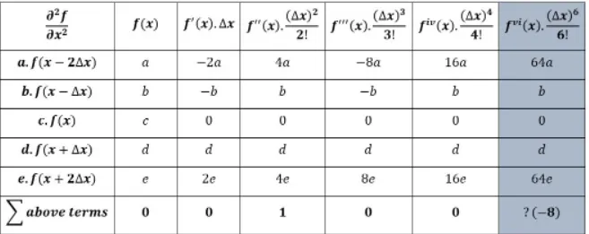
know using this table wa can find the value for the coefficents .

• a+b+c+d+e+g = 0------(1)
• -2adx-bdx+dxd+2edx=0------(2)
• (4a(dx)^2)/2+(b(dx)^2)/2+(d(dx)^2)/2+(4(dx)^2)/2=1--------(3)
• -(8a(dx)^3)/6-(b(dx)^3)/6+(d(dx)^3)/6+(8e(dx)^3)/6=0-------(4)
• (a16(dx)^4)/24+(b(dx)^4)/24+(d(dx)^4)/24+(e(dx)^4)/24=0-----(5).

there for the to nfind the values of a,b,c,d,e from the above tabl we have to write the above tilers tabel content in matrix form of A*X=B.

[1 1 1 1 1 1;-2 -1 0 1 2;2 1/2 0 1/2 2;-8/6 -1/6 0 1/6 8/6;16/24 1/24 0 1/24 16/24][a b c d e]=[0 0 1 0 0 ]

on solving this we can get the value for our coefficents

• a = -0.083333
• b =1.33333
• c=-2.5000
• d=1.3333
• e=-0.08333.

0n distrubuting the values of the co-efficents in equation we will get

(∂^2u)/(∂x)^2=(-0.083333f(i-2)+1.33333bf(i-1)-2.5000f(i)+1.3333f(i+1)-0.0833f(i+2))/(dx)^2

2) deravation for skewed right-side scheme

Nober of node:

n = p+q

n = 4+2

n = 6.

where n is numer of nodes

p is The order of accuracy

q is order of derivative.

using this equation we can draw the diagram for skewed right-side diffrence scheme and our stencil schme look like this

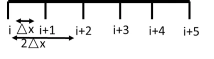
deravation for skewed right-side :

`he main equation for right-sided sheme look like, (∂^2u)/(∂x)^2=af(i)+bf(i+1)+cf(i+2)+df(i+3)+ef(i+4)+gf(i+5)-------(1)

know we have to use the RHS of the above equation and solve this using taylers series we will get below table.

Taylers"s tabel:

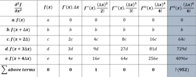
there fore to find the values of a,b,c,d,e from the above tabel we have to write the above tailers tabel content in matrix form of A*X=B.

`[1 1 1 1 1 1 1;0 1 2 3 4 5 ;0 1/2 4/2 9/2 16/2 25/2;0 1/6 8/6 27/6 64/6 125/6;0 1/24 16/24 81/24 25/24 625/24;0 1/120 32/120 243/120 1024/120 3125/120][a b c d e f ]=[0 0 1 0 0 0 ]`

on solving this we can get the value for our coefficents

a =3.7500

b=-12.8333

c=17.8333

d=-13.000

e=5.0833

g=-0.8333.

0n distrubuting the values of the co-efficents in equation we will get

`∂^2u)/(∂x)^2=(3.7500f(i)-12.8333f(i+1)+17.8333f(i+2)-13,000f(i+3)+5.0833f(i+4)-0.85333f(i+50))/dx^2`

now we have to prove that the skewed schems are 4th order accutare

let us take main equation 1 take rhs

`f(i)+bf(i+1)+cf(i+2)+df(i+3)+ef(i+4)+gf(i+5) =f'(i)*dx^2*(a(0)+b/2+4c/2+9d/2+16e/2+25g/2)+f''''''(i)*dx^6(a(0)+b/720+c64/720+729d/720+4096e/720+15625g/720)`

Upon dividing equation above equation by (dx)^2 we get,

we will get

`(f(i)+bf(i+1)+cf(i+2)+df(i+3)+ef(i+4)+gf(i+5))/dx^2 =f'(i)*(a(0)+b/2+4c/2+9d/2+16e/2+25g/2)+f''''''(i)*dx^4(a(0)+b/720+c64/720+729d/720+4096e/720+15625g/720)`

from the above equation we can say thet its a 4th order accurate.

The term denotes the truncation error and the order of approximation. Therefore, the derived equation is of 4th order for the 2nd derivative.

3) deravation for skewed left-side scheme:

Numbers of node :

n = p+q

n = 4+2

n = 6.

where n is numer of nodes

p is The order of accuracy

q is order of derivative.

using this equation we can draw the diagram for left-side diffrence scheme and our stencil schme look like this

deravation for skewed left-side :

`he main equation for right-sided sheme look like(∂^2u)/(∂x)^2=af(i-5)+bf(i-4)+cf(i-3)+df(i-2)+ef(i-1)+gf(i)

know we have to use the RHS of the above equation and solve this using taylers series we can write the below tabel

Tayler's tabel

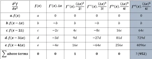
there fore to find the values of a,b,c,d,e from the above tabel we have to write the above tailers tabel content in matrix form of A*X=B.

`[1 1 1 1 1 ;-5 -4 -3 -2 -1 ;25/2 16/2 9/2 4/2 1/2 ;-125/6 -64/6 -27/6 -8/6 -1/6 ;625/24 256/24 81/24 16/24 1/24 ;-3125/120 -1024/120 -243/120 -32/120 -1/120 ][a b c d e ]=[0 0 1 0 0 ]`

on solving this we can get the value for our coefficents

a= -0.8333

b = 5.0833

c=-13.0000

d=17.8333

e=-12.8333

g=3.7500.

0n distrubuting the values of the co-efficents in equation we will get

`(∂^2u)/(∂x)^2=(-0.8333f(i-5)+5.0883f(i-4)-13.0000f(i-3)+17.8333f(i-2)-12.833f(i-1)+3.7500f(i))/dx^2`

now we have to prove that the skewed schems are 4th order accutare

let us take main equation 1 take rhs

`af(i-5)+bf(i-4)+cf(i-3)+df(i-2)+ef(i-1)+gf(i)=;f'(i)*dx^2*(25a/2+125b/2+625c/2+3125d/2+15625e/2)+f'''''(i)*dx^6*(156259a/720+4096b/720+729c/720+64d/720+e/720`

Upon dividing equation above equation by (dx)^2 we get,

we will get

`af(i-5)+bf(i-4)+cf(i-3)+df(i-2)+ef(i-1)+gf(i)) /dx^2= `(f'(i)*dx*(25a/2+125b/2+625c/2+3125d/2+15625e/2)+f'''''(i)*dx^4*(156259a/720+4096b/720+729c/720+64d/720+e/72)dx^2`

from the avove equation we can say thet its a 4th order accurate.

The term denotes the truncation error and the order of approximation. Therefore, the derived equation is of 4th order for the 2nd derivative

4) know we have to write the matlab code for evaluating the 2nd order deravative of the analytic function exp(x)*cos(x)and compare it with the 3 numerical approximation we have derived

code fallows below:

%writting the program for evaluating the given function

clear all
close all
clc

%defining the inputs 
x = pi/3;
dx =linspace(pi/4,pi/4000,20);

for i =1:length(dx)
    error_in_central_deff(i)=central_deravative(x,dx(i));
    error_in_right_hand(i)=right_hand_deravative(x,dx(i));
    error_in_left_hand(i)=left_hand_deravative(x,dx(i));
end
%plotting the graph
%plotting the graph using loglog ploy in order to get the large value
loglog(dx,error_in_central_deff,'color','b')
hold on
loglog(dx,error_in_right_hand,'color','r')
hold on
loglog(dx,error_in_left_hand,'color','g')
hold on
xlabel('schemes')
ylabel('value of dx')
legend('error_central_deff,error_central_deff,error_left_hand')

code for central scheme:

%writting program for evaluating the function exp(x)*cos(x) by central
%deffrence scheme
function error_in_central_deff=central_deravative(x,dx)
% analytic solution for the given function exp(x)*cos(x) 
%f''(x)=-2*sin(x)*exp(x)
analytic_solution=-2*exp(x)*sin(x);
% defing the central deffrence of the iven functin
a = -0.083333;
b =1.33333;
c=-2.5000;
d =1.3333;
e =-0.08333;
central_deffrence =((a*((exp(x-(2*dx)))*(cos(x-(2*dx)))))+((b)*((exp(x-dx))*(cos(x-dx))))+((c)*((exp(x))*(cos(x))))+((d)*((exp(x+dx))*(cos(x+dx))))-((e)*((exp(x+(2*dx)))*(cos(x+(2*dx))))))*(dx^2);
% now taking the error between central deffrence and analytic solution
error_in_central_deff=abs(central_deffrence-analytic_solution);
end

code for right hand skewed sheme

%%writting program for evaluating the function exp(x)*cos(x) by skewed
%%right hand scheme
function error_in_right_hand= right_hand_deravative(x,dx)
% analytic solution for the given function exp(x)*cos(x) 
%f''(x)=-2*sin(x)*exp(x)
analytic_solution=-2*exp(x)*sin(x);
% defing the right hand of the iven functin
skewed_right_hand_deravative=((3.7500)*(exp(x))*(cos(x))-(12.833)*(exp(x+dx))*(cos(x+dx))+(17.8333)*(exp(x+2*dx))*(cos(x+2*dx))-(13.0000)*(exp(x+3*dx))*(cos(x+3*dx))+(5.0833)*(exp(x+4*dx))*(cos(x+4*dx))-(0.8333)*(exp(x+5*dx))*(cos(x+5*dx)))/(dx^2);
% now taking the error between right_hand_deravative and analytic solution
 error_in_right_hand= abs(skewed_right_hand_deravative-analytic_solution);
end

code for left hand skewed sheme

%writting program for evaluating the function exp(x)*cos(x) by skewed
%left hand scheme
function error_in_left_hand=left_hand_deravative(x,dx)
% analytic solution for the given function exp(x)*cos(x) 
%f''(x)=-2*sin(x)*exp(x)
analytic_solution = -2*exp(x)*sin(x);
% defing the left hand of the iven functoin
skewed_left_hand_deravative = (-(0.8333)*((exp(x-(5*dx))*(cos(x-(5*dx))))+((5.0833)*((exp(x-(4*dx)))*(cos(x-(4*dx)))))-((13.0000)*((exp(x-(3*dx)))*(cos(x-(3*dx)))))+((17.8333)*((exp(x-(2*dx)))*(cos(x-(2*dx)))))-((12.833)*((exp(x+dx))*(cos(x+dx))))+((3.7500)*((exp(x))*(cos(x))))))/(dx^2);
% now taking the error between left_hand_deravative and analytic solution
error_in_left_hand=abs(skewed_left_hand_deravative-analytic_solution);
end

output:

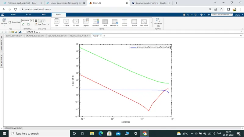
conclustion: from the above graph we can see that central scheme is better then other two schemes becaouse it uses the information from the both side to give approximation and accurate values.

where as in left and right side it usese the information from one side so it failed to give the exact approximation and accurate value \

why a skewed scheme is useful? What can a skewed scheme do that a CD scheme cannot?: cd is cannot be applaid on the baoundry condition becouse there we dnt have left and right point in that case we can apply the left or right schemes inorder to get the results