Week 5.1 - Mid term project - Solving the steady and unsteady 2D heat conduction problem

Aim:

1. Steady state analysis & Transient State Analysis

Solve the 2D heat conduction equation by using the point iterative techniques that were taught in the class. The Boundary conditions for the problem are as follows;

Top Boundary = 600 K

Bottom Boundary = 900 K

Left Boundary = 400 K

Right Boundary = 800 K

You will implement the following methods for solving implicit equations.

1. Jacobi

2. Gauss-seidel

3. Successive over-relaxation

Your absolute error criteria is 1e-4

2. You will write code for both implicit and explicit schemes (This is for the Transient Analysis only).

Answer:

Theory: in this quetion we are going to study the 2-Dheat conduction equation for steady and conduction state of analysis

• firstly we are going to derive the equation for both steady and transient state equation
• after deriving the equation we are going to coding part

1). Steady state: first we have to derive the equation for stedy state condition using fallowing methos

1. jocobian
2. guass sidels
3. saccesive over relaxing (SOR)

there fore we have 2-D heat conduction equation

`(d^2T)/dx^2+(d^2T)/dy^2=0`-----------------(1)

this equation is in the form elliptical in nature, so we are using central scheme deffrencing scheme for solving this equation

there we will get the fallowing equation

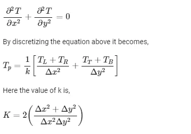
using jacobean scheme we have to derive the deravation

using guass sidels scheme we have to derive the deravation

using seccesive relaxation method we have to derive the deravation

this are deravation fo 2D heat conduction for steady state analysis using jocobian,guass-sidels and succesive over relaxation method

code for steady state analysis fallows below

%writting the program for solving the stedy state analysisi of 2D heat
%conduction equation 

clear all
close all
clc

%defining the inputs as given in the question

%length of the domoin 
L=1;
nx=10;
ny=10;
x=linspace(0,1,nx);
y=linspace(0,1,ny);

% deging the distance betwee the nodes 
dx=x(2)-x(1);
dy=y(2)-y(1);

%defing the boundry conditions 

t=300*ones(nx,ny);
t(1,:)=600;
t(nx,:)=900;
t(:,ny)=800;
t(:,1)=400;

% defining the corners points of the tempreture 
t(1,1)=500;
t(1,ny)=700;
t(nx,1)=650;
t(nx,ny)=850;


%defining the old value 

t_old=t;
%t_prev=t;

%defining the error
error= 100;

%defining the tolerence as given in the question 
tol=1e-4;


%defining the constant value which we have get in the equation 

k= 2*(dx^2+dy^2)/(dx^2*dy^2);

%defing the iterative value 

method=input('iterative_method = ');

%jocobiean method of solving the equation 

if (method==1)
    tic;
    jocobi=1;
    while(error>tol)
        for i=2:nx-1
            for j=2:ny-1
                t(i,j)=(((t_old(i-1,j)+t_old(i+1,j))/(dx^2))+((t_old(i,j-1)+t_old(i,j+1))/(dy^2)))/k;
            end 
        end
        error=max(max(abs(t-t_old)));
        t_old=t;
        jocobi=jocobi+1;
        time_step=toc;
    end
    %ploting the figure 
    figure(1)
    contourf(x,y,t,'showtext','on')
    colormap(jet)
    colorbar
    xlabel('x')
    ylabel('y')
    text_1=sprintf('number of iterstive =%d',jocobi);
    text_2=sprintf('stimulation of time =%f',time_step);
    title({'stedy stete analysis jocobi';text_1;text_2});
end

% soling isung guass sidel method 

if (method==2)
    tic;
    guass=1;
    while(error>tol)
        for i=2:nx-1
            for j=2:ny-1
                t(i,j)=(((t(i-1,j)+t_old(i+1,j))/(dx^2))+((t(i,j-1)+t_old(i,j+1))/(dy^2)))/k;
            end 
        end
        error=max(max(abs(t-t_old)));
        t_old=t;
        guass=guass+1;
        time_step=toc;
    end
    %ploting the figure 
    figure(2)
    contourf(x,y,t,'showtext','on')
    colormap(jet)
    colorbar
    xlabel('x')
    ylabel('y')
    text_1=sprintf('number of iteretive =%d',guass);
    text_2=sprintf('stimulation of time =%f',time_step);
    title({'stedy stete analysis guass';text_1;text_2});
end
% solving using the succesive over relaxing method 

omega=1.4;

if (method==3)
    tic;
    sor=1;
    while(error>tol)
        for i=2:nx-1
            for j=2:ny-1
                t(i,j)=(t(i,j)*(1-omega))+(omega*(((t(i-1,j)+t_old(i+1,j))/(dx^2))+((t(i,j-1)+t_old(i,j+1))/(dy^2)))/k);
            end 
        end
        error=max(max(abs(t-t_old)));
        t_old=t;
        sor=sor+1;
        time_step=toc;
    end
    %ploting the figure 
    figure(3)
    contourf(x,y,t,'showtext','on')
    colormap(jet)
    colorbar
    xlabel('x')
    ylabel('y')
    text_1=sprintf('number of iteretive =%d',sor);
    text_2=sprintf('stimulation of time =%f',time_step);
    title({'stedy state analysis sor';text_1;text_2});
end

Explanetion:

• first we have start the code by writting the cler all close all and clc
• after that we have to derive the expretion for deffrent schmes and then we have to convert that expretion into the matlab code
• then we have to defie the nessary condtion like boundry condition and all other condition
• then we have plot the graph

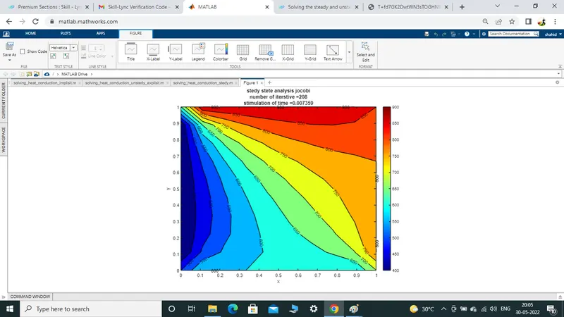
outputs:

for jocobian method

for guass sidels method

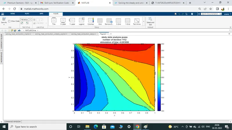
for SOR method

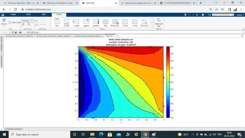
conclustion: a we seen above plots we can clearly say the SOR method give result with less iteative then the other two methods

2) Transient Analysis: in trancient anlaysis we have two schemes fallows below

1. implisit schems
2. explisit schemes.

• implisit scheme: for inplisit schem we have to drive the deravetion using jocobian,guass-sidels and SOR method

deravation for the diffrents fallows below

there fore we have 2-D heat conduction equation

`(d^2T)/dx^2+(d^2T)/dy^2=0`-----------------(1)

this equation is in the form elliptical in nature, so we are using central scheme deffrencing scheme at RHS and forward deffrencing scheme for LHS after solving this equations we will get the fallowing equations

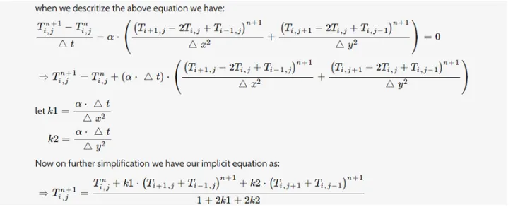
using jacobean scheme we have to derive the deravation

using guass sidels scheme we have to derive the deravation

using seccesive relaxation method we have to derive the deravation

code for implisit method is fallow below

%writting the program for solving the stedy state analysisi of 2D heat
%conduction equation 

clear all
close all
clc

%defining the inputs as given in the question

%length of the domoin 
L=1;
nx=10;
ny=10;
nt=300;
x=linspace(0,1,nx);
y=linspace(0,1,ny);

% deging the distance betwee the nodes 
dx=x(2)-x(1);
dy=y(2)-y(1);

%defing the boundry conditions 

t=300*ones(nx,ny);
t(1,:)=600;
t(nx,:)=900;
t(:,ny)=800;
t(:,1)=400;

% defining the corners points of the tempreture 
t(1,1)=500;
t(1,ny)=700;
t(nx,1)=650;
t(nx,ny)=850;


%defining the old value 
dt=0.01;
t_old=t;
alpha=0.3;
tprev_dt=t_old;

%defining the constant value which we have get in the equation 
error=100;
tol=1e-4;
k_1=alpha*(dt/(dx^2));
k_2=alpha*(dt/(dy^2));
%defing the iterative value 

method=input('iterative_method = ');

%jocobiean method of solving the equation 
if (method==1)
tic;
jocobi =1;
   
    for k=1:nt
        while (error>tol)

        for i=2:nx-1
            for j=2:ny-1
                term_1=(1+(2*k_1)+2*k_2)^-1;
                term_2=t_old(i,j);
                term_3=t(i-1,j)+t(i+1,j);
                term_4=t(i,j-1)+t(i,j+1);
                t(i,j)=((term_1)*(term_2))+((k_1)*(term_1)*(term_3))+((k_2)*(term_1)*(term_4));
               

            end 

        end
        error=max(max(abs(t-t_old)));
        t_old=t;
        jocobi =jocobi+1;
        end
        tprev_dt=t;
    end
         time_step=toc;

     %ploting the figure 
    figure(1)
    contourf(x,y,t,'showtext','on')
    colormap(jet)
    colorbar

    
    xlabel('x')
    ylabel('y')
    text_1=sprintf('iterative_method = %d',jocobi);
    text_2=sprintf('stimulation of time =%f',time_step);
    title({'unstedy stete analysis using explisit ';text_1;text_2});
   
end


%gausian  method of solving the equation 
if (method==2)
tic;
guass =1;
   
    for k=1:nt
        while (error>tol)

        for i=2:nx-1
            for j=2:ny-1
                term_1=(1+(2*k_1)+2*k_2)^-1;
                term_2=t(i,j);
                term_3=t(i-1,j)+t(i+1,j);
                term_4=t(i,j-1)+t(i,j+1);
                t(i,j)=((term_1)*(term_2))+((k_1)*(term_1)*(term_3))+((k_2)*(term_1)*(term_4));
               

            end 

        end
        error=max(max(abs(t-t_old)));
        t_old=t;
        guass =guass+1;
        end
        tprev_dt=t;
        

    end
     time_step=toc;

     %ploting the figure 
    figure(2)
    contourf(x,y,t,'showtext','on')
    colormap(jet)
    colorbar
    xlabel('x')
    ylabel('y')
    text_1=sprintf('iterative_method = %d',guass);
    text_2=sprintf('stimulation of time =%f',time_step);
    title({'unstedy stete analysis using implisit ';text_1;text_2});
 
end

%sor  method of solving the equation 
omega=1.2;
if (method==3)
tic;
sor =1;
   
    for k=1:nt
        while (error>tol)

        for i=2:nx-1
            for j=2:ny-1
                term_1=(1+(2*k_1)+2*k_2)^-1;
                term_2=t(i,j);
                term_3=t(i-1,j)+t(i+1,j);
                term_4=t(i,j-1)+t(i,j+1);
                t(i,j)=((((term_1)*(term_2))*(1-omega))+((omega)*((term_1)*(term_2))+((k_1)*(term_1)*(term_3))+((k_2)*(term_1)*(term_4))));
               

            end 

        end
        error=max(max(abs(t-t_old)));
        t_old=t;
        sor =sor+1;
       
        end
         tprev_dt=t;

    end
     time_step=toc;

     %ploting the figure 
    figure(3)
    contourf(x,y,t,'showtext','on')
    colormap(jet)
    colorbar
    xlabel('x')
    ylabel('y')
    text_1=sprintf('number of itretive = %d',sor);
    text_2=sprintf('stimulation of time =%f',time_step);
    title({'unstedy stete analysis using implisit ';text_1;text_2});
   
end

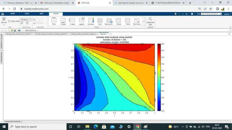
outputs:

for jocobiens method:

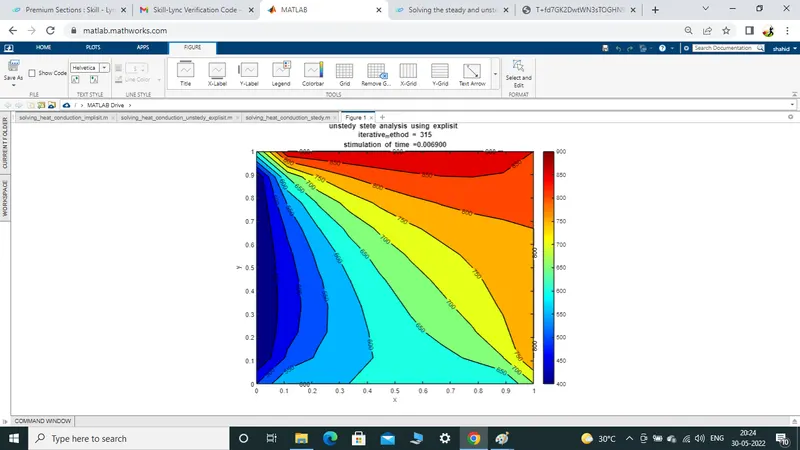
for guass sidels method

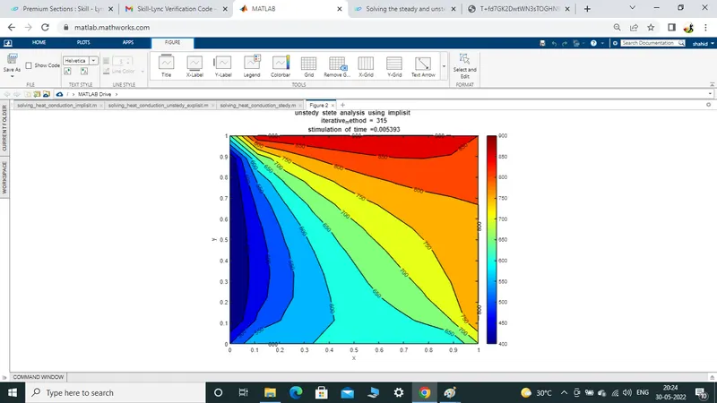
for SOR method

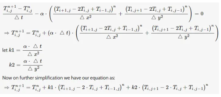
• explisit scheme: here in explisit scheme we have to derive only using central and farwoad schem here we dont need to derive using other 3 methods becouse the valuse for the RHS side expretion we now from earlerly

deravation for explisit fallows below :

code for explisit fallows below:

%writting the program for solving the stedy state analysisi of 2D heat
%conduction equation 

clear all
close all
clc

%defining the inputs as given in the question

%length of the domoin 
L=1;
nx=10;
ny=10;
nt=300;
x=linspace(0,1,nx);
y=linspace(0,1,ny);

% deging the distance betwee the nodes 
dx=x(2)-x(1);
dy=y(2)-y(1);

%defing the boundry conditions 

t=300*ones(nx,ny);
t(1,:)=600;
t(nx,:)=900;
t(:,ny)=800;
t(:,1)=400;

% defining the corners points of the tempreture 
t(1,1)=500;
t(1,ny)=700;
t(nx,1)=650;
t(nx,ny)=850;


%defining the old value 
dt=0.01;
t_old=t;
alpha=0.3;
%t_prev=t;

%defining the constant value which we have get in the equation 

k_1=alpha*(dt/(dx^2));
k_2=alpha*(dt/(dy^2));

%solving the equation  using explisit scheme

explisit =1;
    tic;
    for k=1:nt
        for i=2:nx-1
            for j=2:ny-1
                term_1=t(i-1,j)-2*t(i,j)+t(i+1,j);
                term_2=t(i,j-1)-2*t(i,j)+t(i,j+1);
                t(i,j)=t_old(i,j)+k_1*term_1+k_2*term_2;
            end 
        end
        error=max(max(abs(t-t_old)));
        t_old=t;
        explisit =explisit+1;
        time_step=toc;
    end
     %ploting the figure 
    figure(1)
    contourf(x,y,t,'showtext','on')
    colormap(jet)
    colorbar
    xlabel('x')
    ylabel('y')
    text_1=sprintf('timen= %d',dt*nt);
    text_2=sprintf('stimulation of time =%f',time_step);
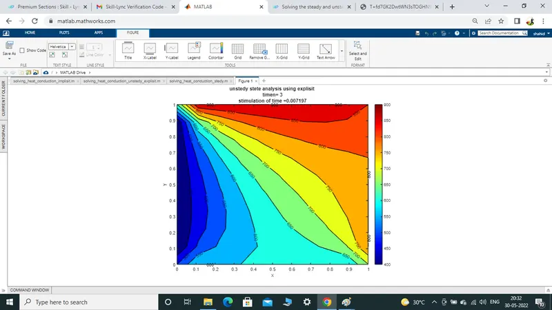
    title({'unstedy stete analysis using explisit ';text_1;text_2});
   

output :