Week-6 Calculate the Stretch Ratio by comparing the ELFORM (-2,-1,1,2) with Ogden_Material Model.
AIM:
Compare the results for the simulation using ELFORM = 1, 2, -1, -2. Plot comparison of various ELFORMS against the Uniaxial Plot.
Objective:
Create a block of 10mmx10mmx10mm dimension with 10 elements for each direction and use the material card attached (Ogden_Material.k) that is representative of the material properties.
Use appropriate boundary conditions to simulate tensile behavior for the model and finally compare the results from your simulation to the plot above up to stretch ratio 5. Only the uniaxial plot is to be compared.
Compare the results for the simulation using ELFORM = 1, 2, -1, -2
The unit of µ in the material definition is in MPa and α is a dimensionless quantity. Modify those quantities according to your unit systems.
Use a proper solver (Implicit/Explicit) and also explain the reason.
PROCEDURE:
1. Create the fea model
2.Define section_solid card
3. Assign the material and section to the part
4.Create boundary conditions
5. Set up the control cards for implicit analysis
6. Request for the plots
7. Model chech
8. Post processing
Explanation:
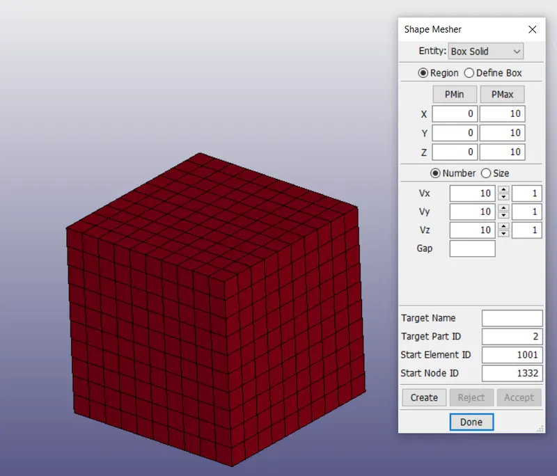
Create a block of 10mmx10mmx10mm dimension with 10 elements for each direction
Go to element and mesh >>> Shape masher >>> Box solid >>> P min (0,0,0) >>> P max (10,10,10) >>> (Vx, Vy, Vz) = (10,10,10).
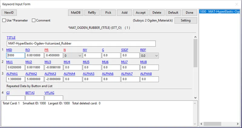
Import the material card attached (Ogden_Material.k) that is representative of the material properties from the below figure.
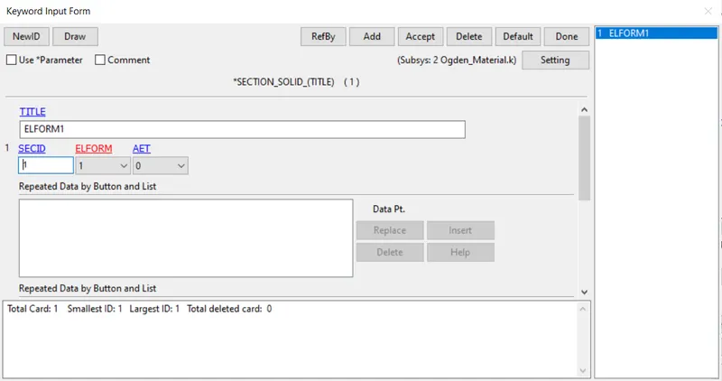
Create the section card using ELFORM = 1
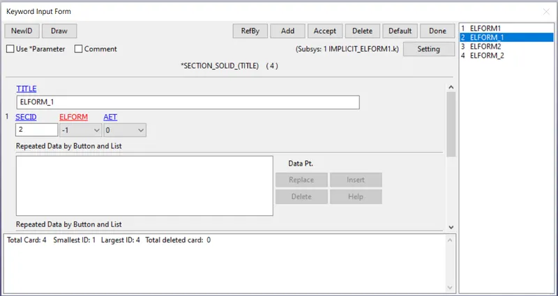
Create the section card using ELFORM = -1
Create the section card using ELFORM = 2
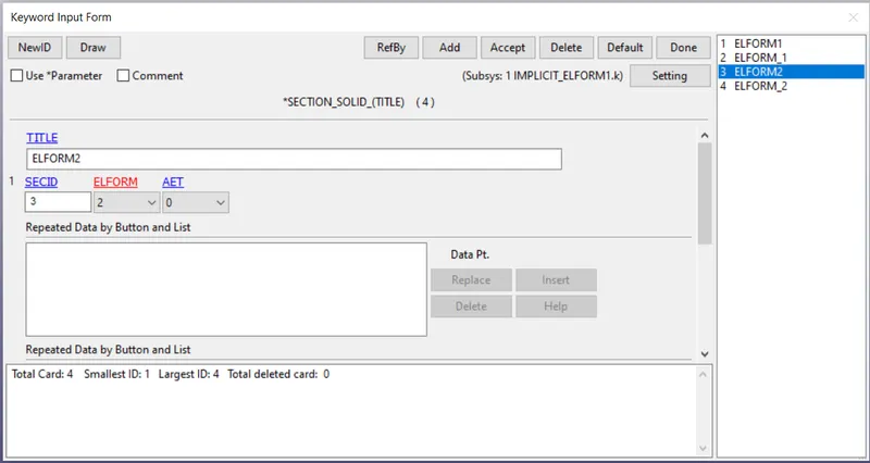
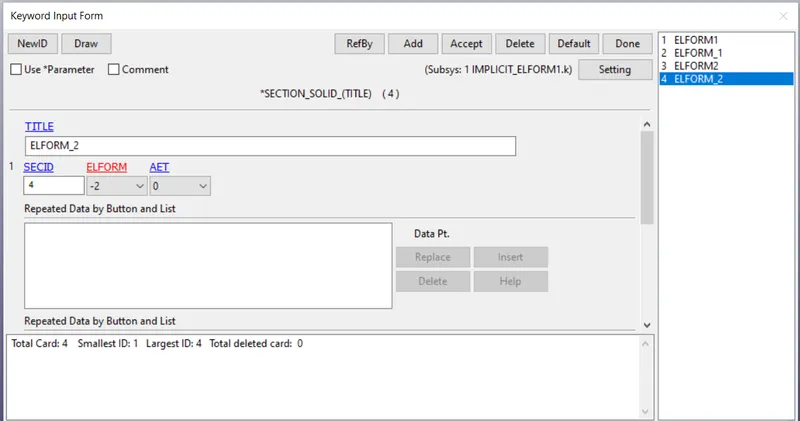
Create the section card using ELFORM = -2
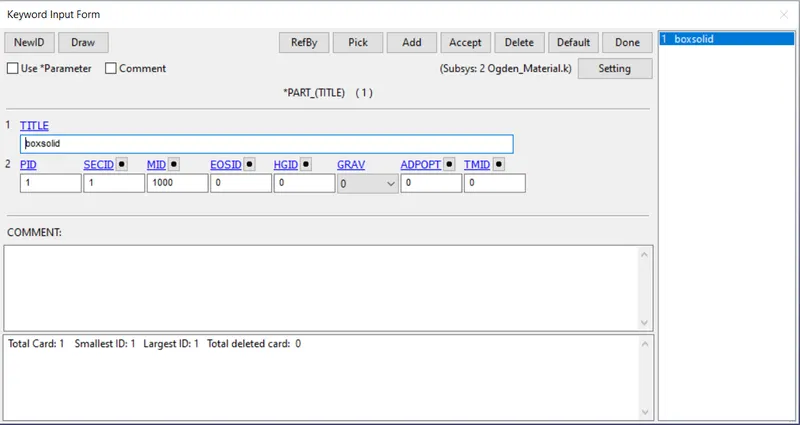
Assign the material and section to the part created.
Use appropriate boundary conditions to simulate tensile behavior for the model:
From the below figure we can see that the compression is happening in y-direction and in the other direction, the lateral strain can be seen in the form of bulging out.
Poissons ratio explains this phenomenon, It is defined as the ratio of lateral strain to the longitudinal strain.
We cannot constrain one side of cube in all degrees of freedom to make it rigid. If we do so, the deformation will be in the tapered manner.
so, we need to constrain in a specific manner as shown below.
1. Constrain all nodes of the side(rigid side) in the x-translation.
there is no need to provide rotational degree of freedom as the 3d elements rotational freedom is always constrained.
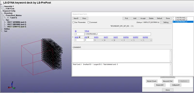
2. constrain the set of nodes as shown below in y-direction. These nodes can move in z-direction.
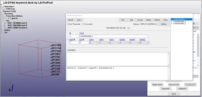
3. constrain the set of nodes as shown below in z-direction. These nodes can move in y-direction.
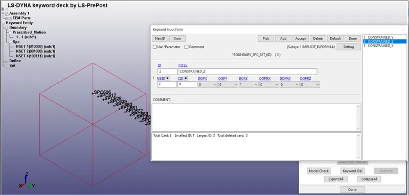
Now, the deformation will take place in a natural way.
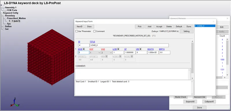
Now, we need to provide the prescribed motion on the other side. the degree of freedom is provided in x-direction by constraining all other sides.
We know that, λ = (1+ engineering strain (ε))
λ = 1+ (change in length/original length)
For the stretch ratio of 5
λ = 5 = 1+ Δl/l (L = 40)
ΔL = 40 mm.
We have to define a curve how displacement is varying over time.
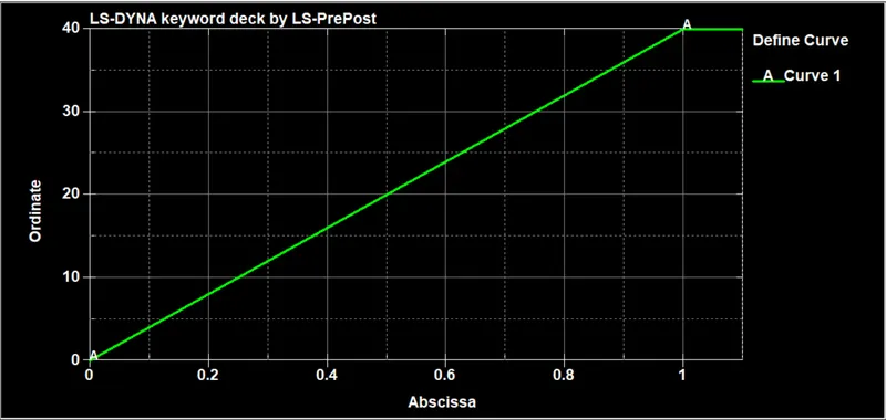
Sf is the scale factor used. if we need to decrease the effect of the load we decrease the value of the scale factor.
Create the control card:
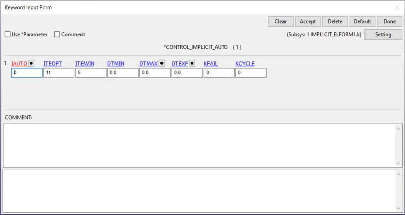
IAUTO = 0 represents the constant time step size.
ITEOPT is the average number of iterations
ITEWIN is the tolerance value
In this case ITEOPT = 11, ITEWIN = 5
It is representing that, if number of interations is in between 6 (11-5) and 16 (11+5) the time step is going to remain constant.
If less than 6, the time step is increased and if more than 16, the time step is decreased.
In our case, we are maintaining the timestep as constant.
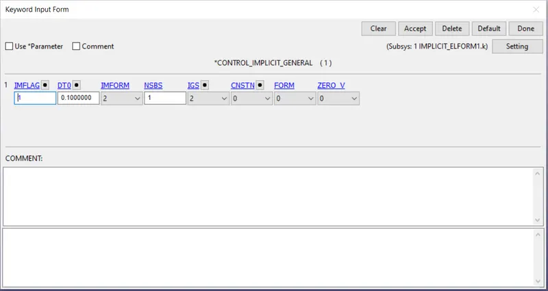
IMFLAG = 1 is activating the implicit solver.
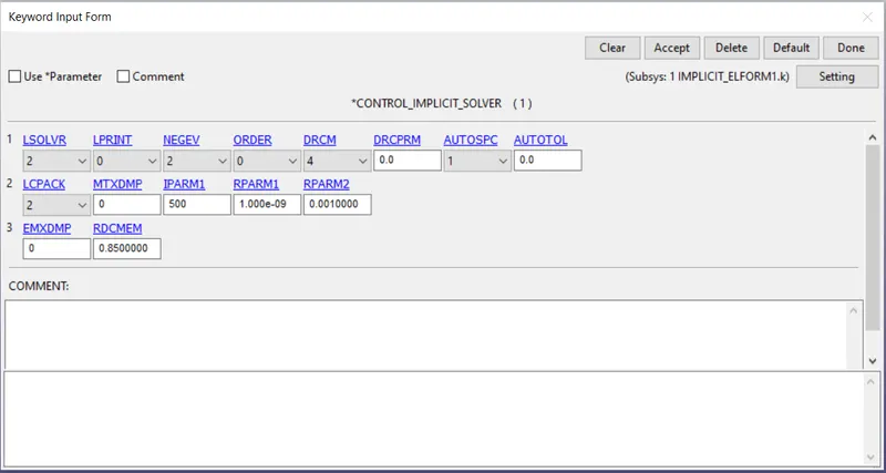
Implicit_Solver is represnting the linear solver
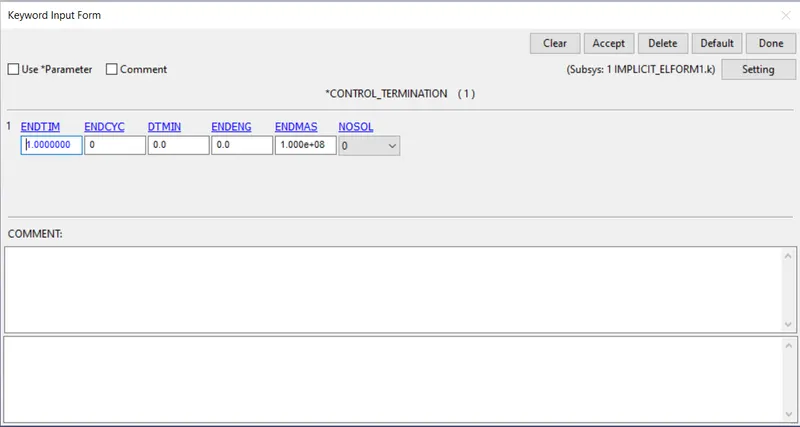
The run time of the simulation is given as 1ms.
Create the database card:
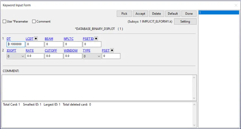
Request for D3PLOT:
DT = 0.1 :Time interval at which the animation files should be printed.
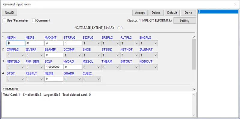
*DATABASE_EXTENT_BINARY Flag for output of strain tensors.
Writes strain tensor data to d3plot and elout.
For shell and thick shell elements two tensors are written, one at the innermost and one at the outermost integration point. For solid elements a single strain tensor is written.
Model check:
After assigning all the keywords, Check the model using model checker and make sure that the file is error free.
After model checkup, save the file in .k format and run the simulation
Results:
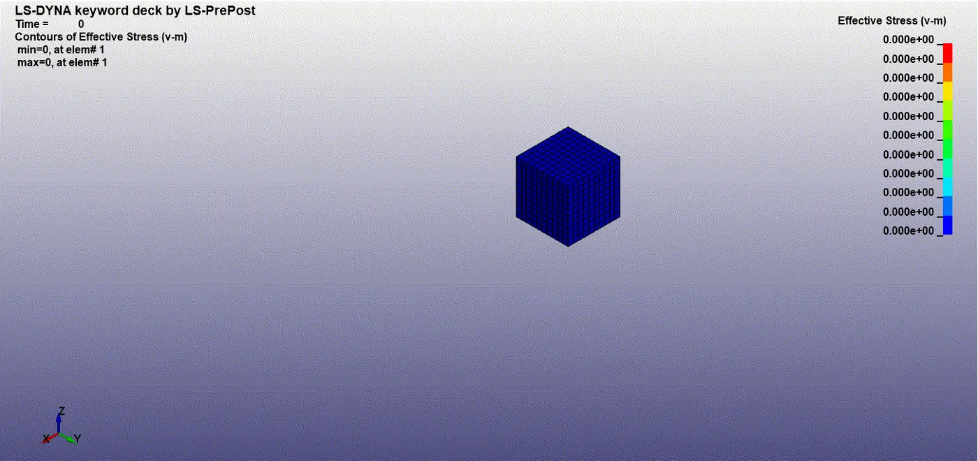
ELFORM = 1
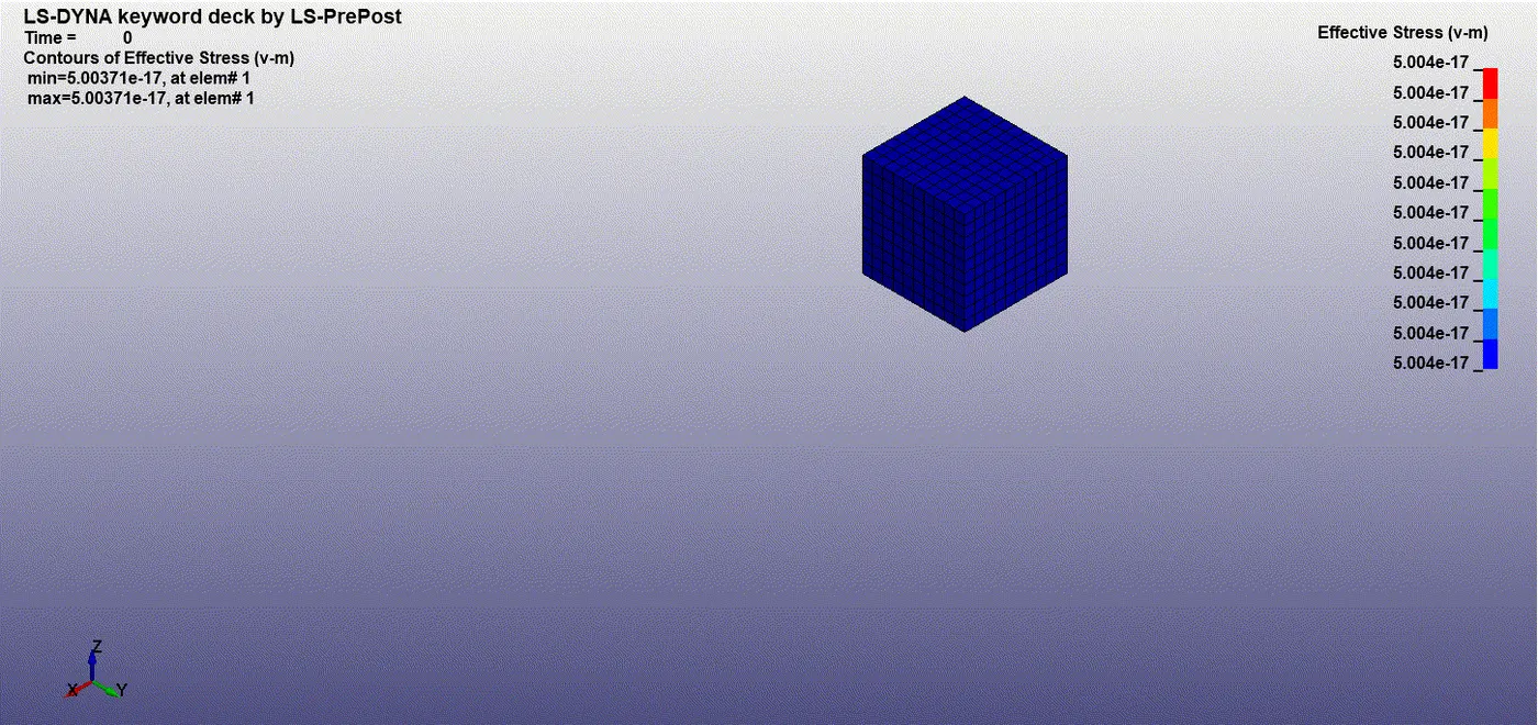
Effective stress by using ELFORM = 1
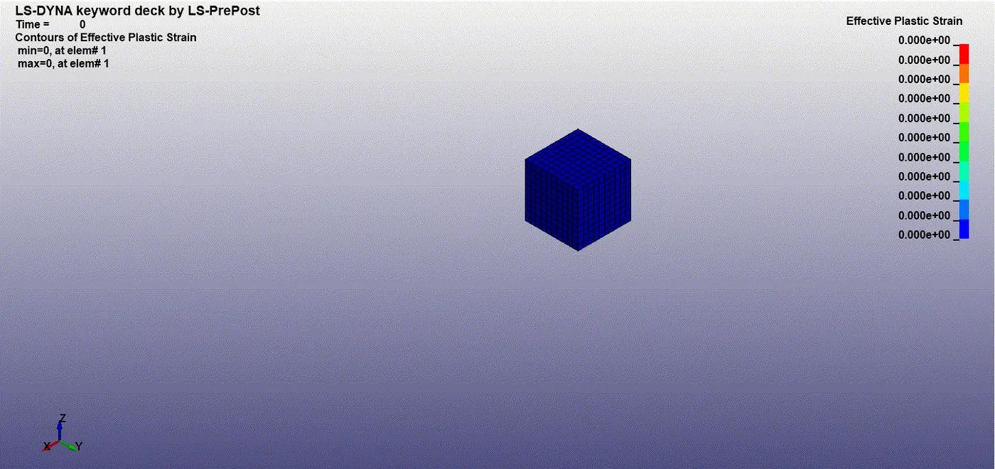
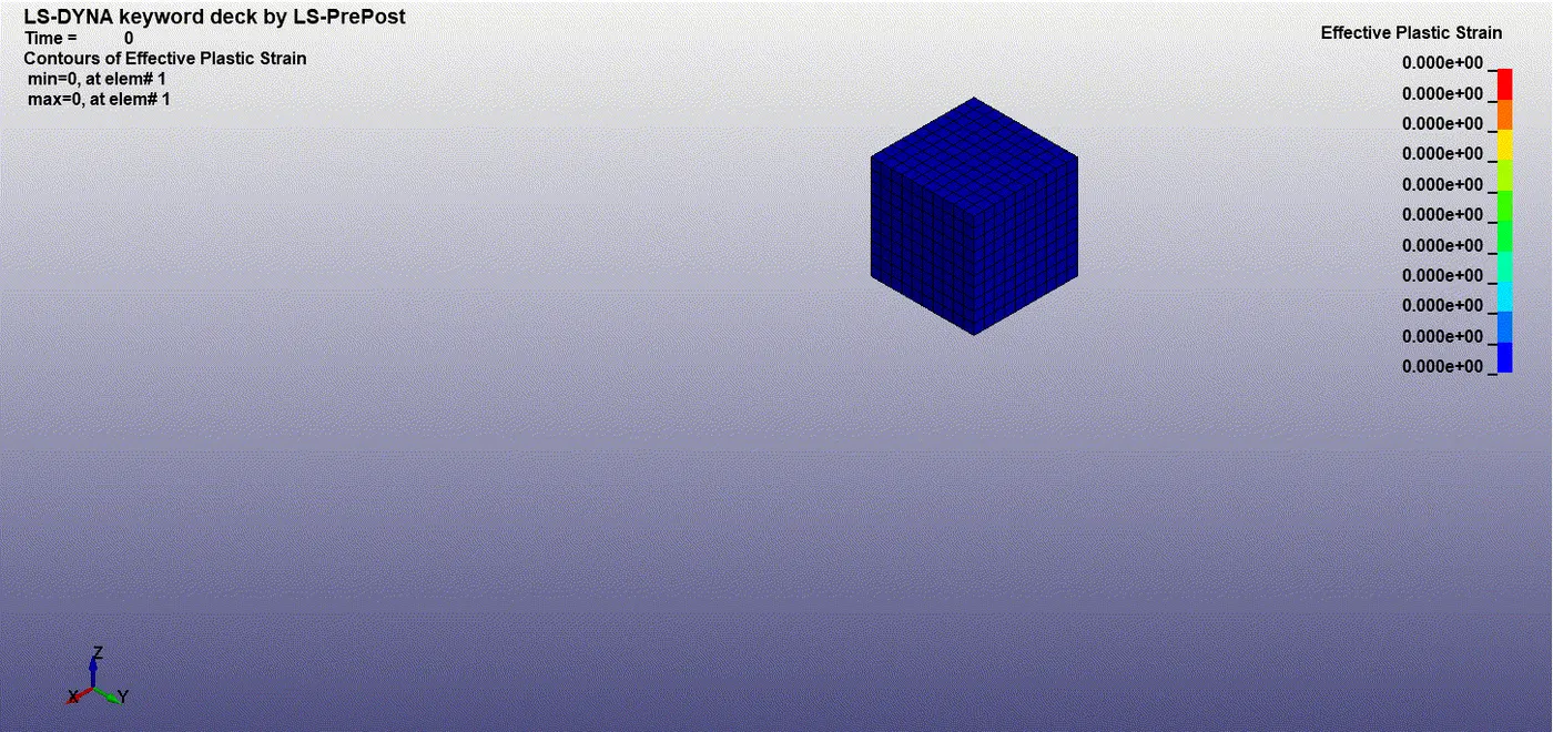
Effective Plastic strain by using ELFORM = 1
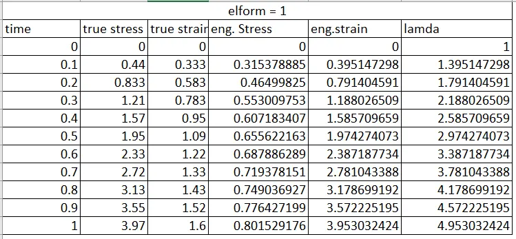
The table representing stress, strain and stretch ratio for ELFORM = 1
ELFORM = 2
Effective stress by using ELFORM = 2
Effective Plastic strain by using ELFORM = 2
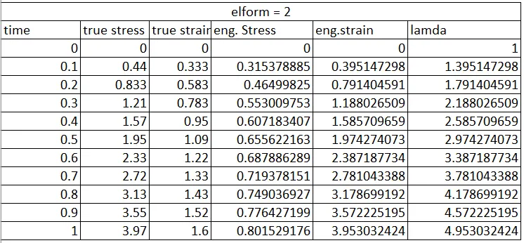
The table representing stress, strain and stretch ratio for ELFORM = 2
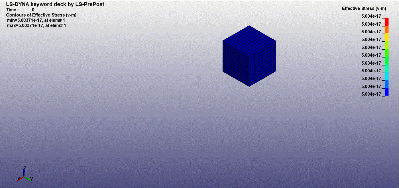
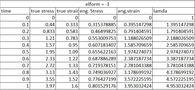
ELFORM = -1
Effective stress by using ELFORM = -1
Effective Plastic strain by using ELFORM = -1
The table representing stress, strain and stretch ratio for ELFORM = -1
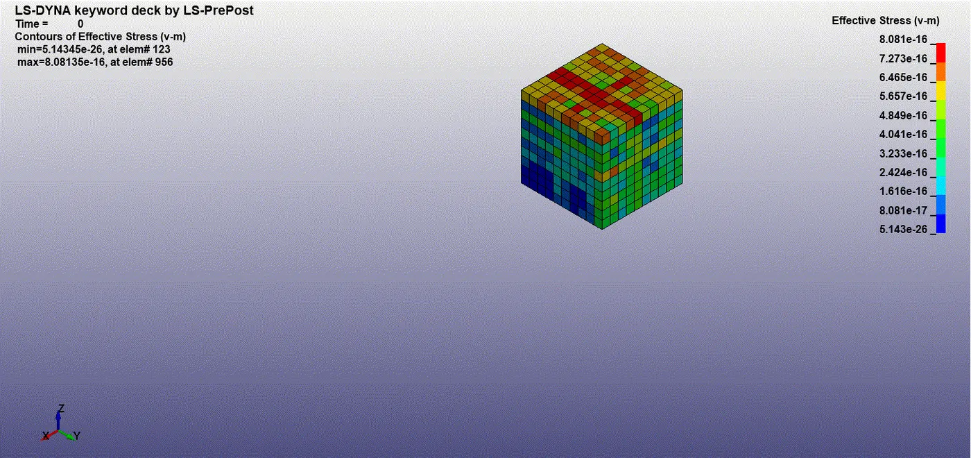
ELFORM = -2
Effective stress by using ELFORM = -2
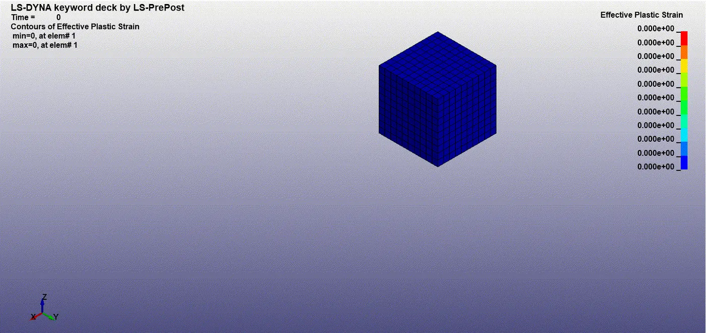
Effective Plastic strain by using ELFORM = -2
The table representing stress, strain and stretch ratio for ELFORM = -2
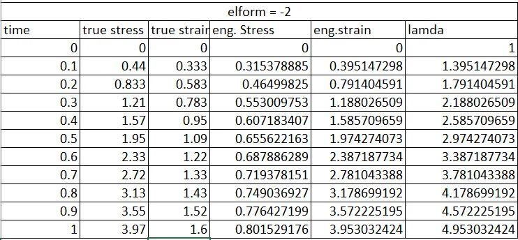
Calculation of engineering stress, engineering strain and stretch ratio:
ε true = ln (1+ε.eng)
σ true = σ eng (1+ε.eng)
λ = 1+ (change in length/original length)
λ = 1+ ε.eng
ε T = ln(λ)
σ eng = σ true / λ
The Engineering Stress and the stretch values that we got from the Elform 1, -1, 2, -2 are same.
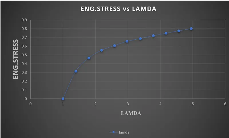
We have plotted a graph graph of engineering stress vs Lamda from the values obtained from calculation.
Conclusion:
Based on our study, we conclude that the stress vs lamda are constant for ELFORM = 1, -1, 2, -2. For our simpler problems we can't see any difference from the varying elform 's, We can see a difference when a complex problem is the case. The suitable elform is to be choosen in that case depending on the problem.
Element Formulation ID provides the appropriate shell formulation.
EQ.0: 1 point corotational for *MAT_MODIFIED_HONEYCOMB,
EQ.-2: fully integrated S/R solid intended for elements with poor aspect ratio, accurate formulation.
EQ.-1: fully integrated S/R solid intended for elements with poor aspect ratio, efficient formulation.
EQ.1: constant stress solid element (default),
EQ.2: fully integrated S/R solid,
EQ.3: fully integrated quadratic 8 node element with nodal rotations,
EQ.4: S/R quadratic tetrahedron element with nodal rotations,
EQ.5: 1 point ALE,
EQ.6: 1 point Eulerian,
EQ.7: 1 point Eulerian ambient, EQ.8: acoustic,
EQ.9: 1 point corotational for *MAT_MODIFIED_HONEYCOMB,
EQ.10: 1 point tetrahedron,
EQ.11: 1 point ALE multi-material element,
EQ.12: 1 point integration with single material and void,
EQ.13: 1 point nodal pressure tetrahedron for bulk forming,
EQ.14: 8 point acoustic,
EQ.15: 2 point pentahedron element,
EQ.16: 5 point 10 noded tetrahedron;
EQ.17: 10-noded composite tetrahedron
EQ.18: 8 point enhanced strain solid element for linear statics only,
EQ.19: 4 point cohesive element,
EQ.20: 4 point cohesive element with offsets for use with shells,
EQ.21: 6-noded, 1 point pentahedron cohesive element.
EQ.22: 6-noded, 1 point pentahedron cohesive element with offsets for use with shells.
EQ.23.: 20-node hexahedron formulation.
EQ.24.: 27-node hexahedron formulation.
EQ.25.: 21-node pentahedron formulation
EQ.26.: 15-node tetrahedron formulation
EQ.41: Mesh-free (EFG) solid formulation
EQ.42: Adaptive 4-noded mesh-free (EFG) solid formulation
EQ.43: Mesh-free enriched finite element
EQ.45: Tied Mesh-free enriched finite element
EQ.47: Smoothed particle Galerkin method
EQ.98: Interpolation solid
EQ.99: Simplified linear element for time-domain vibration studies,
EQ.101-105: User defined solid.
EQ.115: 1 point pentahedron element with hourglass control.
GE.201: Isogeometric solids with NURBS. (See *ELEMENT_SOLID_NURBS_PATCH)