Week-6 Calculate the Stretch Ratio by comparing the ELFORM (-2,-1,1,2) with Ogden_Material Model.

Skill-lync assignment 6

Aim: The objective of this assignment is to create an FE model with the material card provided and simulate tensile behavior in said model using a suitable explicit/implicit solver. The model is to be solved in multiple iterations with different element formulations and the results are to be compared.

Case setup: The material provided is rubber defined by the MAT>77_O-OGDEN_RUBBER keyword with the following parameters (changed from gm mm ms to kg mm ms units) defined:

• Density (RO): 1 X 10^-6 kg/mm³
• Poisson’s ratio (PR): 0.45
• First shear modulus (MU1): 6.2 X 10^-4 GPa
• Second shear modulus (MU2): 1.18 X 10^-6 GPa
• Third shear modulus (MU3): -9.81 X 10^-6 GPa
• Αlpha 1: 1.3
• Alpha 2: 5
• Alpha 3: -2

The model is to be worked on in iterations, where each one uses solid elements with one on the following element formulations: -

1. 1 (constant stress solid element)
2. 2 (fully integrated S/R solid)
3. -1 (fully integrated S/R solid intended for elements with poor aspect ratio, accurate formulation)
4. -2 (fully integrated S/R solid intended for elements with poor aspect ratio, efficient formulation)

The model will be solved using implicit analysis. This decision is based on the priority of an accurate stress/strain plot without concern for any dynamic model behavior.

Expected deliverables: The following output are required from this assignment: -

• Excel sheet with stress vs. strain data and conversion of strain to stretch ratio.
• Plot of stress vs. stretch ratio for various element formulations.

Procedure: The model is prepared through the following sequence of steps.

1. The keyword file containing the material card is imported into the LS-PrePost workspace.
2. The parameters in the keyword file are converted to kg, mm, ms units, as mentioned in the case setup.
3. Using the shape mesher tool, a cube with side 10 mm divided into cubical elements with side 1 mm is generated.
4. A solid section card is generated with element formulation of 1 (constant stress solid element), which is then assigned to the part, along with the material.
5. The create entity tool is used to create 3 constraints at one face of the component. One constraint locks movements of all the nodes in the face in the x-direction. The second constraint locks the movement of two nodes in the opposing faces in the other directions, along with rotation about the x axis. The final constraint locks movement in the y direction in the face on which displacement is applied.
6. A displacement curve is defined by the DEFINE_CURVE keyword. The curve is a linear ramp of load up to 1 mm at time t=50 ms.
7. The create entity tool is used to set a prescribed displacement in the x direction on the opposite face. A scale factor of 40 is applied to bring the value of displacement to 40 mm.
8. The CONTROL>IMPLICIT_GENERAL keyword is edited to use implicit analysis for the model (IMFLAG: 1) with a time step (DT0) of 0.5 ms.
9. The CONTROL>TERMINATION keyword is edited so that run time is 50 ms and minimum time step is 0.5 ms.
10. The DATABASE>BINARY_D3PLOT keyword is edited so that the d3plot output file is generated with a time step of 0.5 ms.
11. The model checker is then run to check for errors/discrepancies in the model.
12. The simulation is then run in the LS-Run to generate output files.
13. The d3plot is imported into the LD-PrePost workspace.
14. The energy plot is then checked for discrepancies that might suggest faults in the model definition.
15. The maximum effective Von Mises stress history is output into an excel (XML) file.
16. The stretch ratio in this model is given by dividing the maximum x coordinate of the model by the initial value of the same, i.e. 10 mm. This is achieved by changing the scale factor for the plot to 0.1 and multiplying the upper and lower limits by this value. The resultant plot is then output as an excel file.
17. Three copies of the keyword file are created. In the first copy, the element formulation is changed to 2 (fully integrated S/R solid). In the second copy, it is changed to -1 (fully integrated S/R solid intended for elements with poor aspect ratio, efficient formulation). In the third copy, it is changed to -2 (fully integrated S/R solid intended for elements with poor aspect ratio, accurate formulation).
18. These files are individually simulated and the steps 13-15 are repeated for each iteration.
19. The stretch ratio and the various stress history plot files are loaded into an X-Y plot to generate the final stress vs. stretch ratio in an excel file.

Results: The following observations were made from the assignment: -

• The Energy plot for all the iterations show practically no kinetic energy and a parabolic increase in internal energy, as shown in the image below.

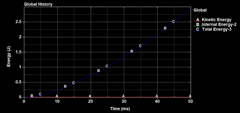
Figure 1: Energy plot

Since the internal and total energy are almost identical, this indicates that there are no discrepancies in the element formulations. The parabolic profile also indicates linear stress behavior in the model.

• The final stress vs. stretch ratio plot is illustrated below.

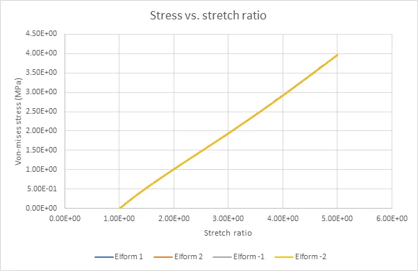
Figure 2: Stress vs. stretch ratio plot computed

It shows virtually no difference in the computed stress and stretch ratio values between all the element formulations. This could be attributed to the decision to use the implicit solver to simulate the model. The inherent residual reduction in this solver reduces the variation in the final solution, thus reducing the necessity of stringent element formulation. The resultant plot is a nearly linear one with barely noticeable slopes. It also bears little resemblance to the original plot provided, shown below.

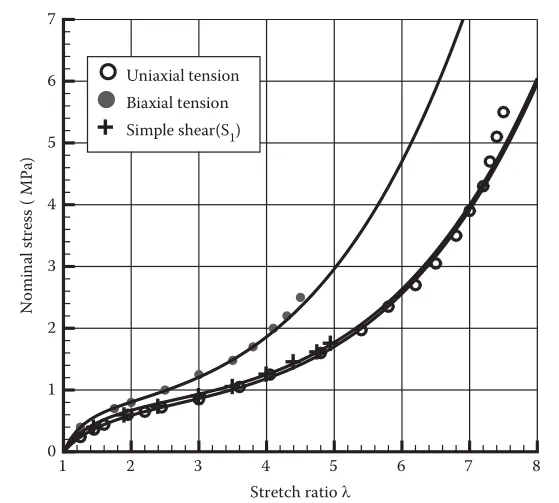
Figure 3: Actual stress vs. stretch ratio plot for given material

This might be due to the stretch ratio demanded being too low to demonstrate otherwise. Judging by this graph, if the stretch ratio required were to be up to 7, there might have been some noticeable increase in slope for the computed plot.

Conclusion: The model has been successfully simulated with the stipulated element formulations. The required stress vs. stretch ratio plots were computed, but no variations could be observed between the iterations involved.