Week-6 Calculate the Stretch Ratio by comparing the ELFORM (-2,-1,1,2) with Ogden_Material Model.

AIM: In this challange given Ogden Material card which is hyperelastic (Rubber). We have to create a 10X10X10 mm solid mesh and run on it with stretch ratio of 5. Compare different element formulations of solids 1,-1,2,-2 and polt engineering stress vs stretch value.

EXPLANATION:

This simulation is happening at a really slow pace (Quasi Static) the inertial effects can be neglected we can consider implicit for the analysis.

As the material is Hyper elastic material even though we are running it in implicit, we need steps and iterations to achive the equilibrium.

ELFORM used are as follows:

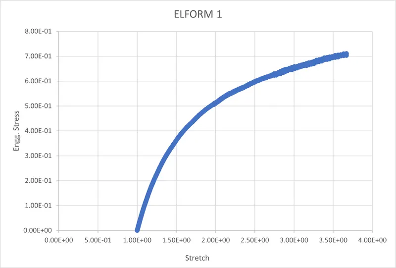
CONDITION-1 : ELEMENT FORMULATION_1

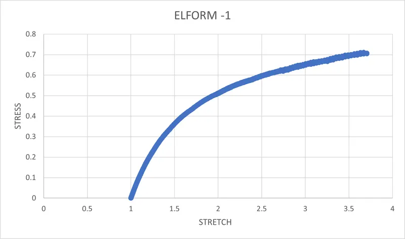
CONDITION-2 : ELEMENT FORMULATION_-1

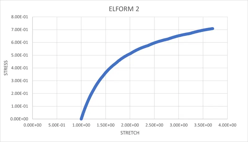
CONDITION-3 : ELEMENT FORMULATION_2

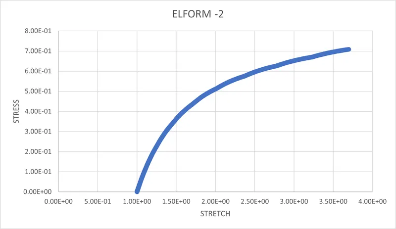
CONDITION-4 : ELEMENT FORMULATION_-2

PROCEDURE:

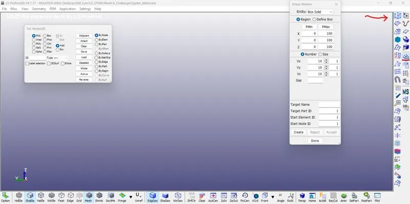
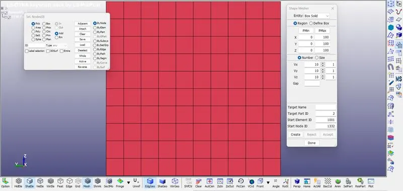
• Firstly we will load the file in LS-DYNA then we will create the 10x10x10 box in LS-DYNA under Element and Mesh then Shape Mesher.
• After that we will be entering all the values in X,Y and Z direction in order to create cube, then click on create and accept option to creating a Box.

Section:

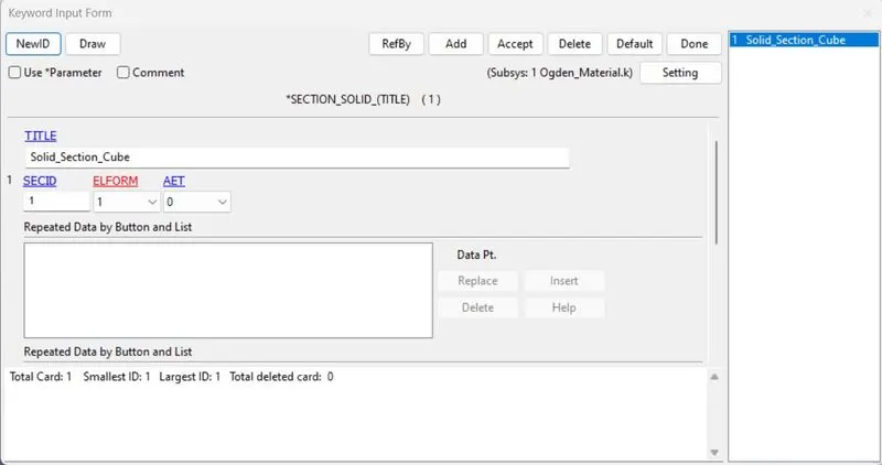
• After creating Cube of 10X10X10 now we will be assigning the Section for the cube and also assingning the element formulation criteria as per given condition that is it will be -1,1,2 & -2.

Material Properties:

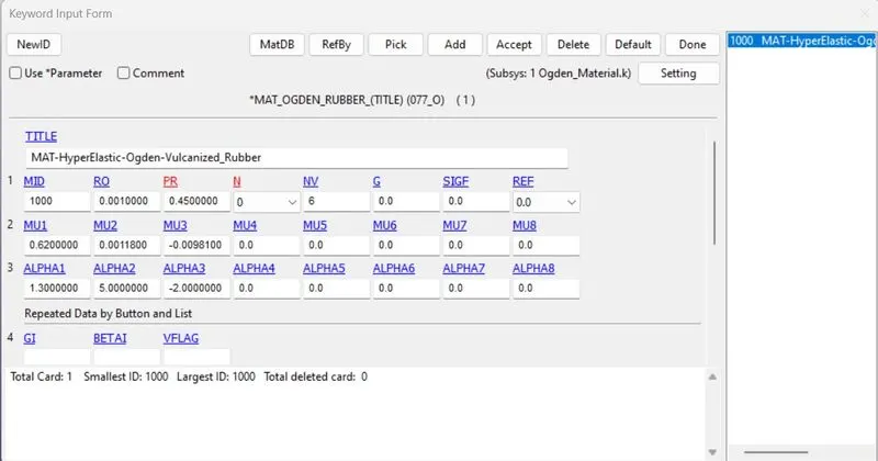
• Material Property card for the ogden material model which was given.

Part:

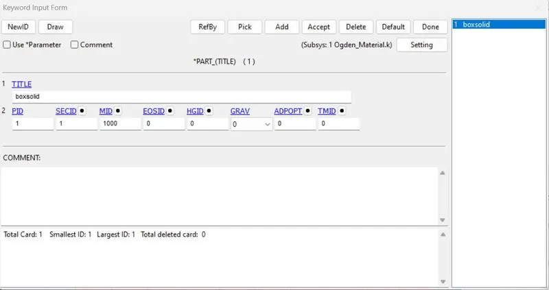
• Now we will creating part id assigning sectionid and material id in part.

Boundary Condition:

• We will fix the bottom of the cube and given the motion to the set of nodes on upper face.
• To fix the bottom face, we will use different set of nodes and using single point constraint boundary, we can allow or constraint the nodes with different DOF.

Single Point Constrained:

• Boundary Conditions using single point constrained for different set of nodes will be as given below:

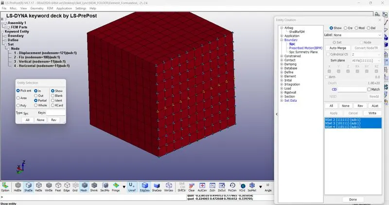
• For this challange we will create 3 SPCs one is in vertical direction with having z-axis and x-axis fixed, second is in horizontal direction with having y-axis and x-axis fixed and third is in rest other nodes in face fixed in all axis.

Prescribe Motion:

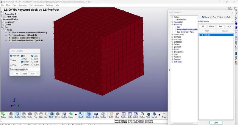
• We will provide prescribe motion in positive x direction and for achiving stretch ratio of 5.

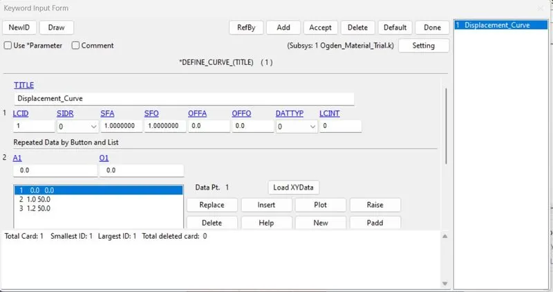
• Motion is given to the node set in the form of curve as given. And displacement is given is of 50mm.

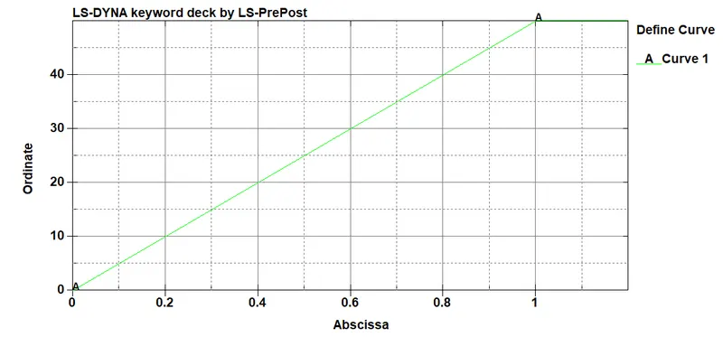
• After difining curve we will assign the load curve to the prescribed motion card.

Control Card:

• LS-DYNA employs both implicit and explicit methods to solve static, quasi-static and dynamic problems.
• These problem can differ in time increment approach.
• To make sure that LS Dyna runs the model in implicit analysis control implicit cards need to be defined.
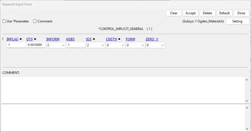
• Implicit general then parameter IMFLAG=1 in order to activate the implicit analysis method and time step value is given DTMIN (Initial Time Step size)= 0.001ms is given.

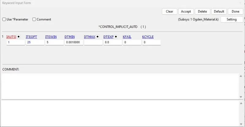
• Implicit auto card is used so that the solver can change the time step size as needed automatically.(Manual Control of iteration per each step ITEOPT)

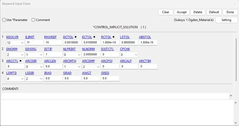
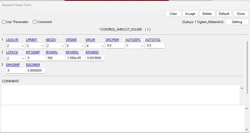
• Control Implicit Solution here Nsolver is set to 12 as the material is very non linear in nature and displacment tolerance is set to 0.001,Implicit solver default parameters are used.

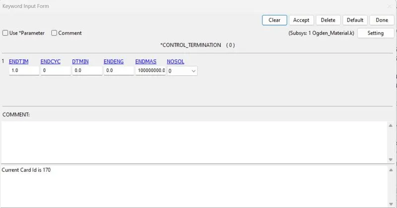
• We will also assign Control_Termination,ENDTIM is set to 1. Here termination does not represent the time but gives the value at which step the analysis will end.

Database:

• Now we will define DATABASE_EXTENT_BINARY it is used to get strain tensor data through D3PLOT.

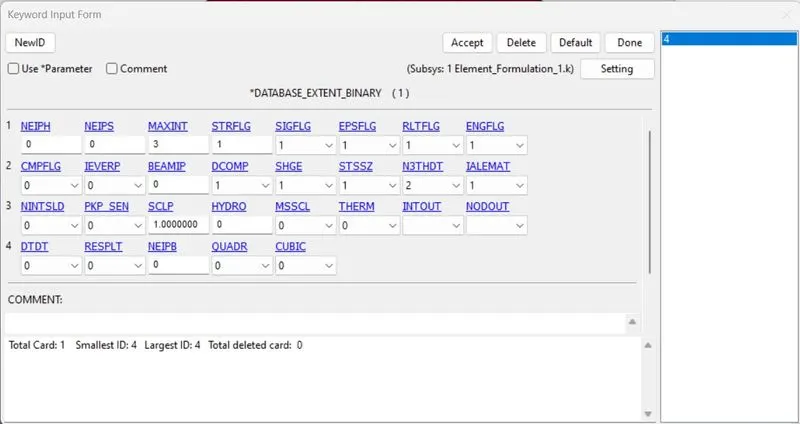
• Similarly DATABASE_BINARY_D3PLOTkeyword is used for all output data and animations.

Results:

• We will plot graph with the help of history and selecting strain in X-direction and Effective stress.
• Firstly we will be selecting effective stress the plotting the graph and then selecting X-Strain and pressing new option.
• With the help of XY plot we will combine both graphs from cross.

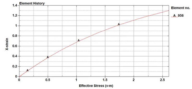
As we know the relationship-

True Stress= Engg. Stress(1+Engg. Strain)

True Strain= ln (1+ Engg Stain)

Stretch= (1+Engg. Strain)

• For taking out reading to excel we will be saving the above graph in Msoft (Microsoft) CSV format. Which is Excel format which will help in plotting the graph.

Conclusion:

• There is not much considerable difference in stress values between formulation for stretch value of 5.
• Usage of different element formulation depends on accuracy or efficiency that is CPU time requirements.
• In this condition a large variation could not be found, when model is large enough we can notice a significant difference in the computational time.