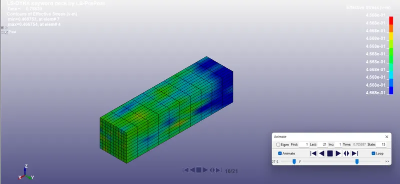
Week-6 Calculate the Stretch Ratio by comparing the ELFORM (-2,-1,1,2) with Ogden_Material Model.

Introduction

The Ogden material model is a hyperelastic material model used to describe the non-linear stress-strain behavior of complex materials such as rubbers, polymers, and biological tissue. The model was developed by Raymond Ogden in 1972. The Ogden model, like other hyperelastic material models, assumes that the material behavior can be described by means of a strain energy density function, from which the stress-strain relationships can be derived.

For modeling rubbery and biological materials at higher strains, the more sophisticated Ogden material model has been developed.

Analysis

Here we will perform a simple tensile test on a 10x10x10 mm cube with the Ogden material model.

To see the behavior of element formulation, we will work on different cases as per different element formulations as given below:

CASE_1: Element Formulation_ (1)

CASE_2: Element Formulation_ (2)

CASE_3: Element Formulation_ (-1)

CASE_4: Element Formulation_ (-2)

_____________________________________________________________________________________________________________________

Geometry

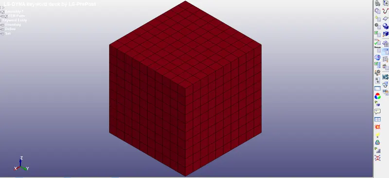
Procedure:

• First of all, open the L S DYNA Keyword file named “Ogden_Material.k” in LS-PrePost.
• Create a cube of 10x10x10 mm with help of “Shape Mesher” in “Elements and Mesh” as shown below:

• As per the above image, give the value 10 for x, y, and z directions and create a cube.

Material Properties

The material properties for the Ogden material model will be as given below:

 

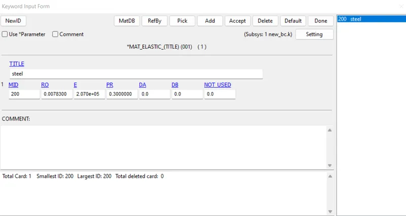
Section:

• Create a Section card for the cube and assign the element formulation criteria as per the case as given below:
• As per the case, as shown in the above image, element formulations will be 1, 2, -1, and -2.

 

Part:

• After the creation of Sections and Materials, we have to assign them to the Part.

Assignment of appropriate material as well section in part for all cases will be a given below:

Boundary Conditions:

• Here we will fix the Bottom of the Cube and give the motion to the set of nodes on the Upper face.
• To fix the Bottom face, we will use a different set of nodes, and using a single point constraint boundary, we can allow or constrain the nodes with different degrees of freedom.

Single Point Constrained:

• Boundary conditions using a single point constrained for a different sets of nodes will be as given below:

        

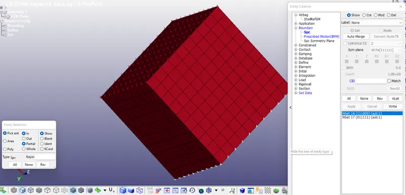
• As shown in the above image, constraints are given for the different sets of nodes in a way that the cube can shrink in X and Y directions upon tension in Z-Direction and also stick to its position.

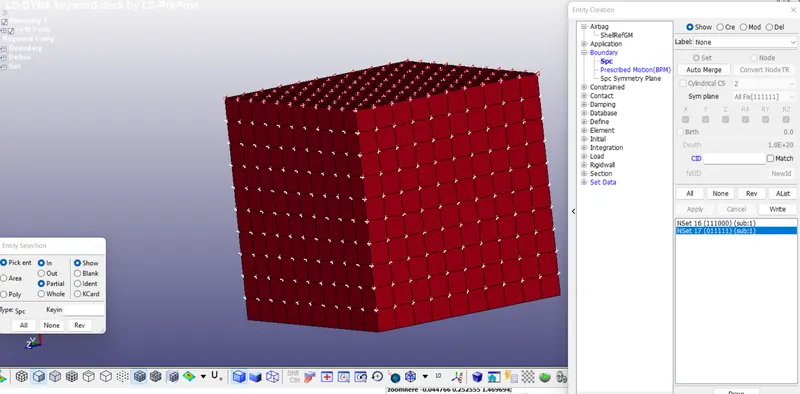
• Thus, this boundary condition can be relatable to the real-time boundary condition.

Prescribed Motion:

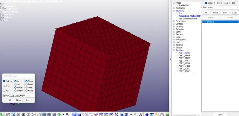
• To apply the tensile load in Z-Direction to the cube, we have to give the motion to the set of nodes on the upper face of the cube.

• As per the above image, motion is given to the set of nodes of the cube on the upper face.
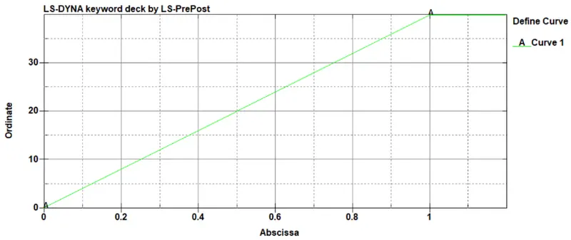
• Motion is given to the node set in the form of a curve as given below:

• After defining the proper curve, assign the load curve to the Prescribed motion card as given below:

• As shown in the above image, we have given DOF = 3, to allow translation in Z-Direction translation
• VAD = 2 is given for Displacement.
• A load curve is also assigned for the desired displacement.
• As we have given the curve for the 1 mm displacement, the Scale Factor is set to 50 for displacement up to 50 mm.

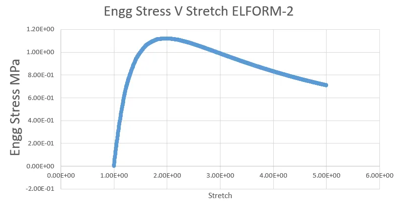
Here we want to obtain the stretch ratio up to 5.

Stretch is the ratio of Final length to Original length.

So, to obtain the stretch ratio up to 5,

Original length = 10 mm

Final length = 50 mm

So, Stretch ratio = Final length/ Original length = 50/10 = 5.

• So, to get the stretch ratio up to 5, we have given the displacement up to 50 mm.

Analysis Method:

LS-Dyna employs both implicit and explicit methods to solve Static, Quasi-Static, and Dynamic problems.

These problems can differ in the Time Increment approach.

• In implicit each Time increment has to converge, but we can set quite long time increments.
• In explicit, convergence for each time step is not needed.
• In the implicit method, at each time increment, global equilibrium is established, due to the iterative method.
• The implicit method is used for accuracy and can be applied for long-duration problems.
• Also, implicit methods are used when the deformation is not so large or the deformation is happening in a gradual manner.
• Here, we stretched the cube up to 50 mm, which is large deformation, but for the hyperelastic materials, this deformation can be small.
• So, an implicit scheme is best for this type of analysis.

Control:

Since this is the nonlinear implicit analysis, we need to create some implicit cards to activate implicit methods like implicit auto, implicit general, etc as given below:

• In *CONTOL_IMPLICIT_GENERAL, IMFLAG =1 is given to activate the implicit analysis method and the initial Time step value is given as 0.01.
• In *CONTROL_IMPLICIT_AUTO, values of DTMIN and DTMAX are not defined, so the solver can change the time step size as needed automatically.
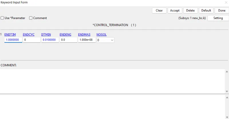
• In CONTROL_TERINATION, ENDTIME is set to 1. Here termination does not represent the time but gives the value at which step the analysis will end.

Results

We know relationship (before necking)    => True stress = Engg stress ( 1 + engg strain)

                                                           => True Strain = ln ( 1 + engg strain) = ln (stretch)

                                                           => Stretch = 1 + engg strain 

Post-processing plotting x stress and mean x strain for all the Element formulations, true stress and strain can be found.

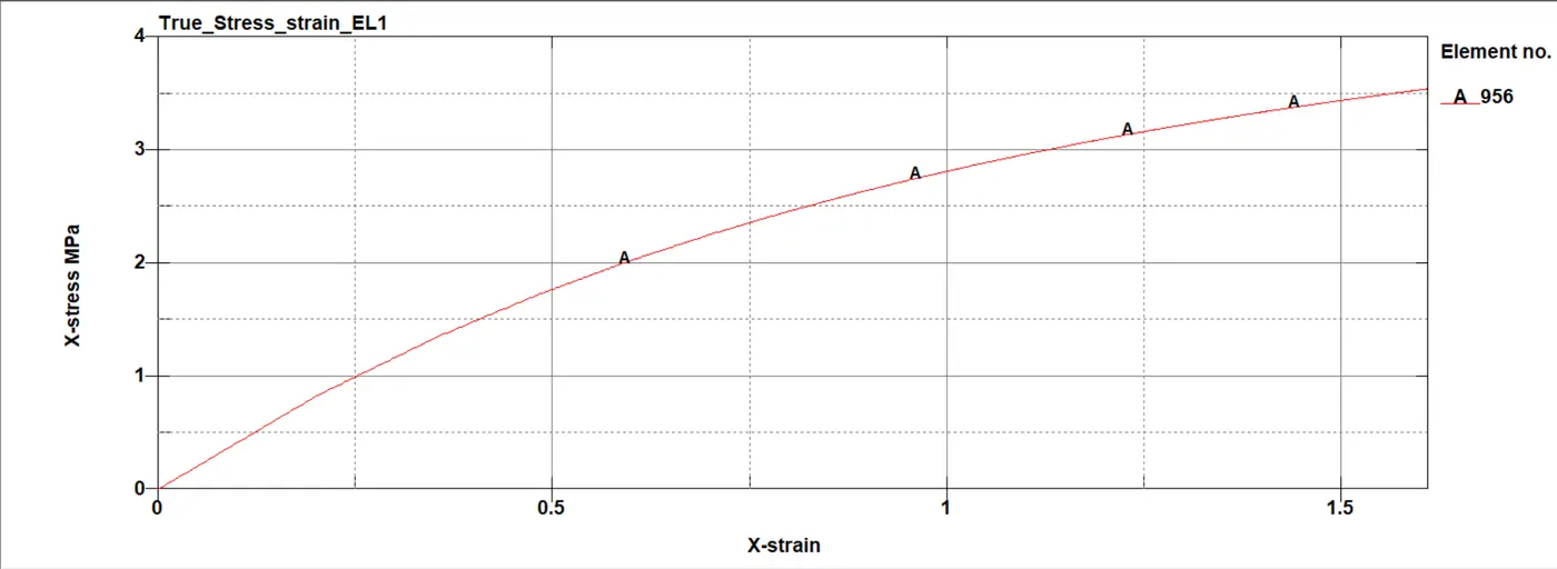
- The above graph is a true uniaxial (x) stress-strain curve of the Ogden material with ELFORM 1 from ls dyna.

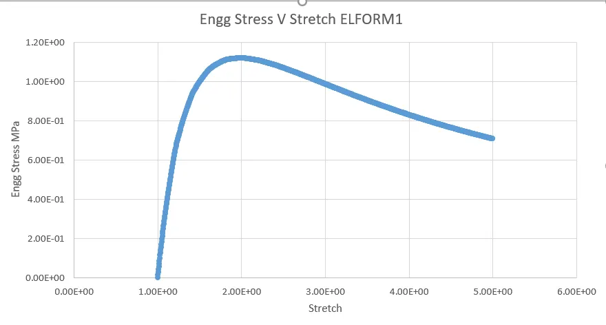
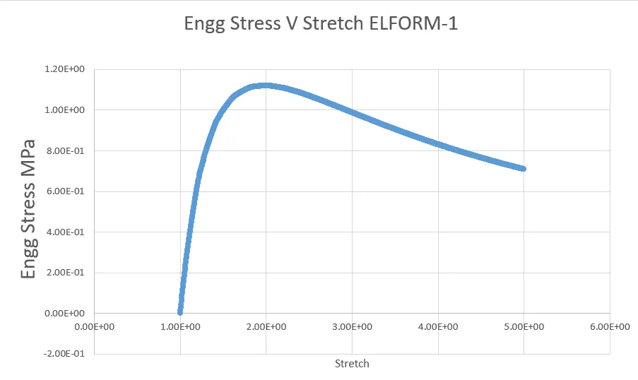
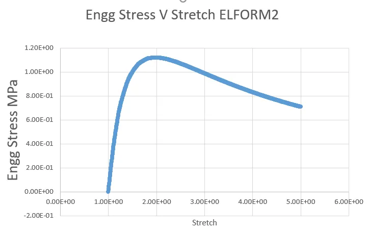
- From this Engg stress and strain > then stretch ratio can be found out.

- Using excel the Engg stress and stretch ratio can be compared.

Von mises Stress :