Week-6 Calculate the Stretch Ratio by comparing the ELFORM (-2,-1,1,2) with Ogden_Material Model.

Calculate the Stretch Ratio by comparing the ELFORM (-2,-1,1,2) with Ogden_Material Model

OBJECTIVE:-

1) To create a block of 10mmx10mmx10mm dimension with 10 elements for each direction and use the material card attached (Ogden_Material.k) that is representative of the material properties from the above figure.

2) To use appropriate boundary conditions to simulate tensile behavior for the model and finally compare the results from the simulation to the plot above up to stretch ratio 5. Only the uniaxial plot is to be compared.

3) To compare the results for the simulation using ELFORM = 1, 2, -1, -2. Th e unit of µ in the material definition is in MPa and α is a dimensionless quantity.

4) To use a proper solver (Implicit/Explicit) and also explain the reason.

INTRODUCTION:-

An Ogden model is a hyperelastic material model that can be used for predicting the nonlinear stress-strain behaviour of materials such as rubber or polymer. Ogden model was introduced by Ogden in 1972. Ogden model has been frequently used for the analysis of rubber components like O-ring and seal. This material model is generally used for material showing incompressible, isotropic and non-linear stress-strain behaviour. Even though Ogden model is a hyperelastic material model, its strain energy density function is expressed by principal stretch ratio.

A solid cube of rubber material modelled by Ogden material model is simulated for tensile behaviour. Different Element Formulations are used to compare stress versus stretch behaviour. The solver used for this simulation is implicit solver because the analysis is similar to a quasi-static analysis on a hyperelastic non-linear material with slow steady loading conditions.

Implicit vs. Explicit Method:-

Implicit method is choosen over Explicit method. It is because of the following reasons -

1. The tensile behaviour of the cube is time-dependent and slow process, where inertial effects are not much important. Explicit method are suitable for solving fast process where inertial effects will be taken into consideration.
2. Implicit method solves the problem directly by inverting stiffness matrix. Ogden material has a non linear stress-strain behaviour and hence this cannot be solved in one step, but equilibrium iterations would help to solve the problem which is carried out in Implicit Method.

UNIT SYSTEM:- gm mm ms

PROCEDURE:-

1) Import the .k file:-

The given keyword file is opened in LS-PrePost using the option File > Open > LS-Dyna Keyword file. The file consists of only one Material card which is *MAT_OGDEN_RUBBER.

2) Model Creation:-

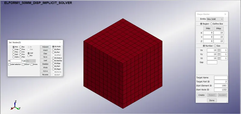
Create a Finite Element Model of a solid block of 10mm x 10mm x 10mm with 10 elements for each direction as shown in the figure. Go to Mesh > ShapeMesher > Entity: Box Solid > Given the required dimensions as shown in the figure > Click on create > Done.

3) MAT Card:-

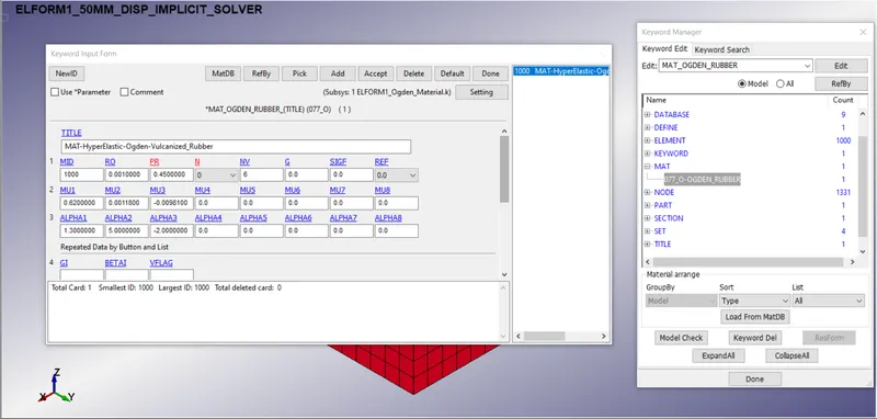
Review the material properties which was given along with keyword file: A separate material card has been created named *MAT_OGDEN_RUBBER which is used to define the non-linear behaviour of materials like rubber and polymers. Here µ and α are constants and the unit of µ in the material definition is in gm/mm.ms^2 and α is a dimensionless quantity.

4) Defining Section Card:-

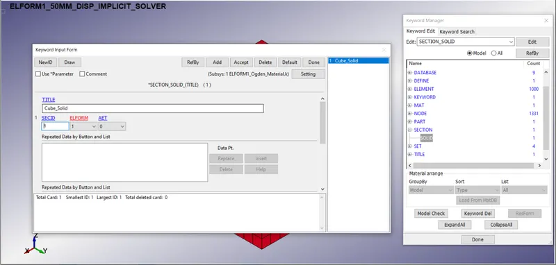
Scetion card is defined for the rubber material cube by going to SECTION_SOLID.

The section properties of the FE model created is assigned as a solid element with different ELFORM -

Case (1). ELFORM = 1, constant stress solid element.

Case (2). ELFORM = -1, Fully integrated S/R solid intended for elements with poor aspect ratio, efficient formulation.

Case (3). ELFORM = 2, Fully integrated S/R solid

Case (4). ELFORM = -2, Fully integrated S/R solid intended for elements with poor aspect ratio, accurate formulation.

• S/R - Selected Reduced

5) Part Definition:-

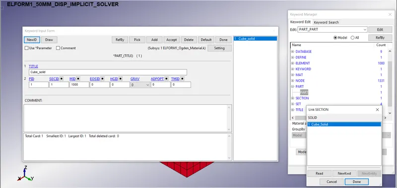
The material cards and section cards which have been defined, should be assigned to the respective parts in *PART card.

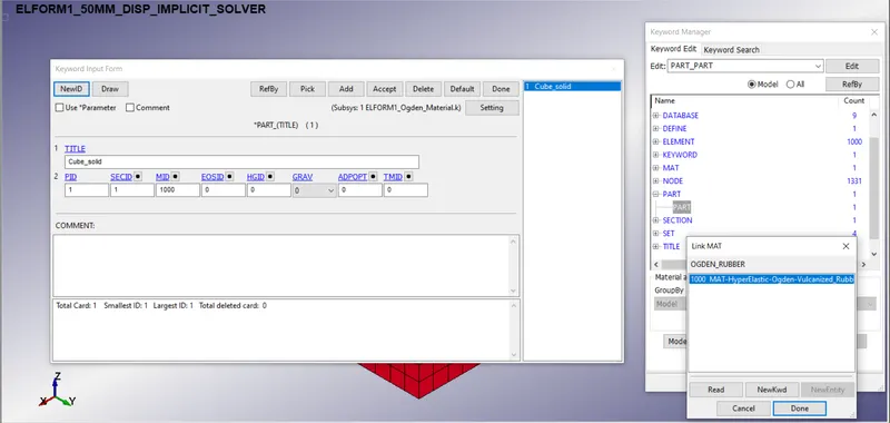
6) Boundary Conditions:-

• Creating Node Sets:-

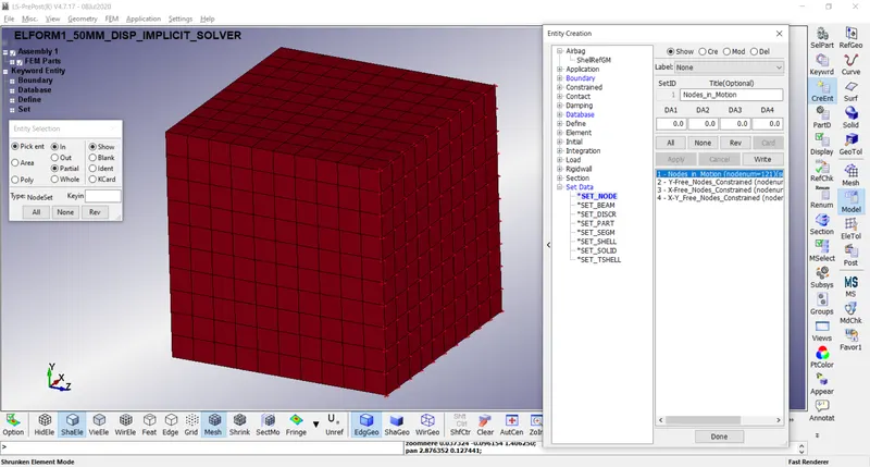
For creating the node sets, go to Model > Create Entity > Set Date > *SET_NODE > Create.

1) For Prescribed Motion:-

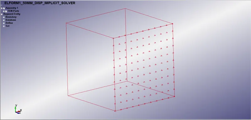
Here in this simulation, we need to simulate tensile behavior for the model so we have define motion for a set of nodes present at the face normal to the direction in which we want to stretch the rubber cube and in this case it is the face, normal to the z-direction.We have created a node set by title Nodes_in_Motion for Prescribed Motion.

2) For Single Point Constraints:-

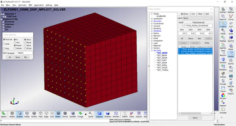
Here we have created 3 node sets for SPC so that different types of constraints can be defined for different sets of nodes.

• Defining Motion Curve:-

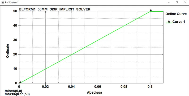
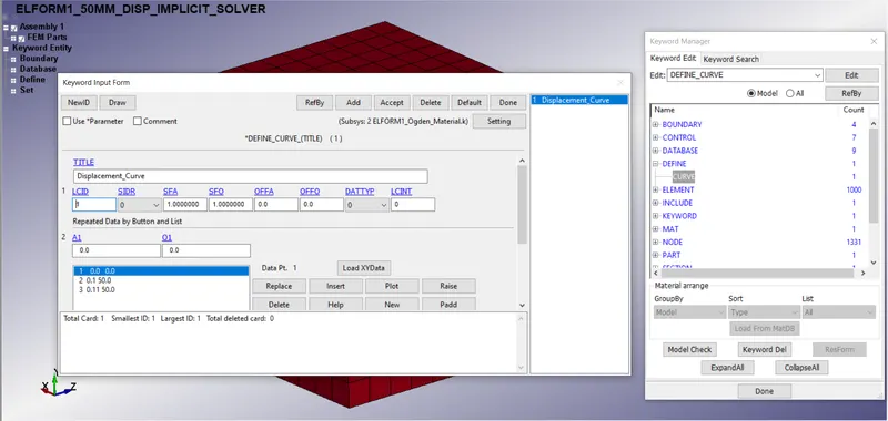
A motion Curve has to be defined for specify motion for the node set and it can be defined by going to DEFINE_CURVE.

The minimum load to be applied on the moving surface to attain a stretch ratio of 5, is calculated by using the following relation -

True strain = ln (1+Engg.strain)

Stretch Ratio = 1+Engg.strain

5 = 1+ ( delta L / L )

delta L = 40 mm

Hence, the minimum value of 40mm is taken to define the load curve.

As we want the simulation to last for 0.1ms so the max. time is 0.1ms and the max displacement it can get is 50mm.

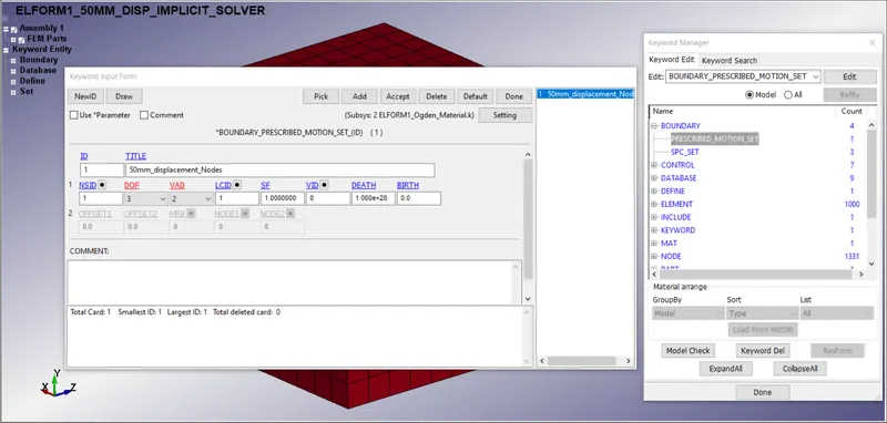
• PRESCRIBED_MOTION_SET Card:-

This card is defined for nodes to give them prescribed motion so NSID and LCID are given as input here which we have already created.

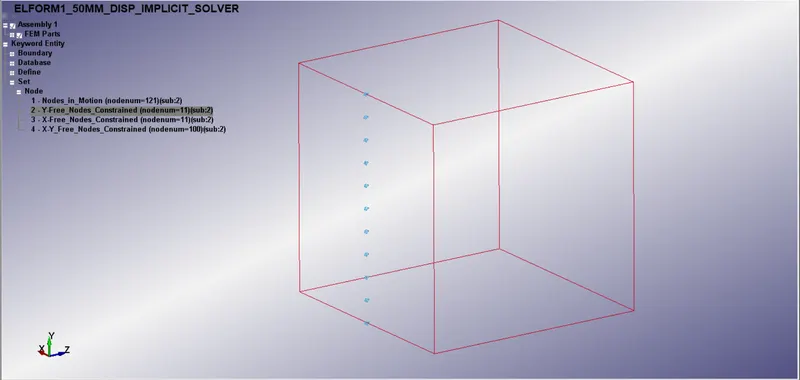
• SPC_SET Card:-

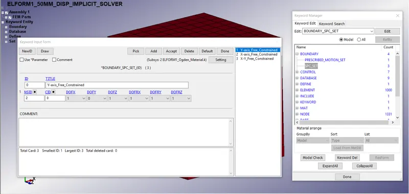
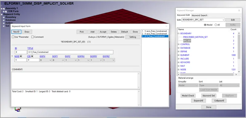
Total 3 SPC Sets are defined here and DOFs are given to them accordingly -

1 Y-axis _Free_Constrained: This node set is defined for the nodes along Y-axis at middle fibre of the face opposite to the face which is having Prescribed Modtion Set nodes. Here this node set is allowed to move in Y-direction only in order to encounter the decrement in lateral dimension while pulling the face of the cube in Z-direction.

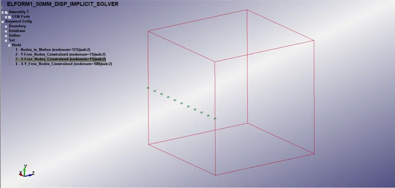
2 X-axis _Free_Constrained: This node set is defined for the nodes along X-axis at middle fibre of the face that is opposite to the face which is having Prescribed Modtion Set nodes. Here this node set is allowed to move in X-direction only in order to encounter the decrement in lateral dimension while pulling the face of the cube in Z-direction.

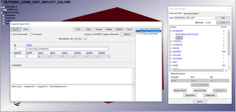
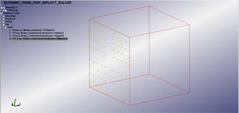
3 X-Y_Free_Constrained: This node set is defined for all the remaining nodes at the face that is opposite to the face which is having Prescribed Modtion Set nodes. Here this node set is allowed to move in both X-Y direction in order to encounter the decrement in lateral dimensions while pulling the face of the cube in Z-direction.

7) CONTROL Keyword:-

Some of the important control cards which is used in Implicit analysis are shown below -

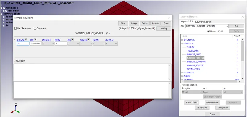
• *CONTROL_IMPLICIT_GENERAL:

It is used to activate Implicit analysis and define associated control parameters. This card is required for all types of Implicit analysis. Input value for Implicit/Explicit switching flag (IMFLAG) = 1 and Initial time step size (DTO) for implicit analysis is 0.005ms.

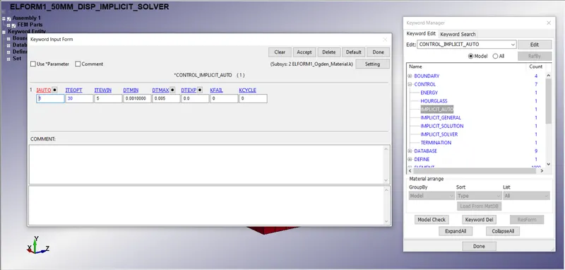
• *CONTROL_IMPLICIT_AUTO:-

It is used for automatic time step control during Implicit analysis. Input value for Automatic time step control flag (IAUTO) is set as 1.

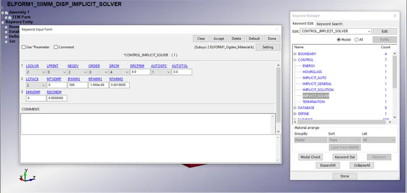
• *CONTROL_IMPLICIT_SOLVER:-

This keyword is for linear solver parameters and used for implicit calculations.

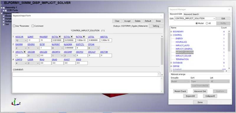
• *CONTROL_IMPLICIT_SOLUTION-

This keyword is used to specify whether a linear or non-linear solution is desired. This keyword is for non-linear solver parameters.

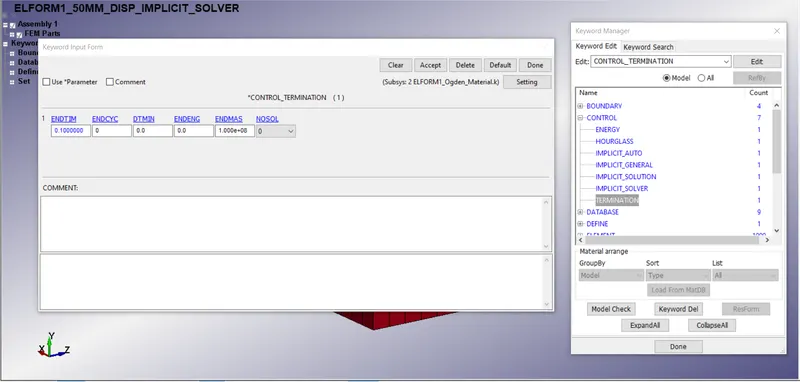
• *CONTROL_TERMINATION:-

It is enabled to specify the end time of the simulation and termination time is set for 0.1ms.

8) DATABASE Keyword:-

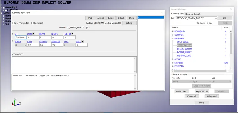
• *DATABASE_BINARY_D3PLOT:-

It is used to get the outputs. Time step should be given as 0.005ms.

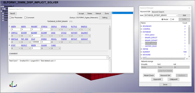
• *DATABASE_EXTENT_BINARY:-

It is used to compute elastic strain in the model and some of the strain data. STRFLG should be given as 1.

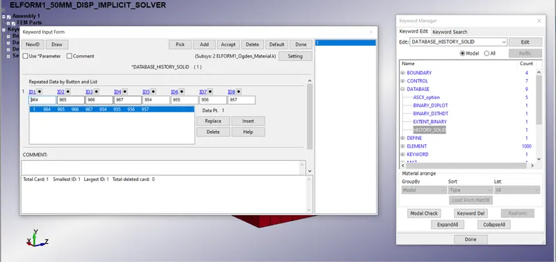
• *DATABASE_HISTORY_SOLID:-

It is used to compute stress/strain in the model at 966 th Element.

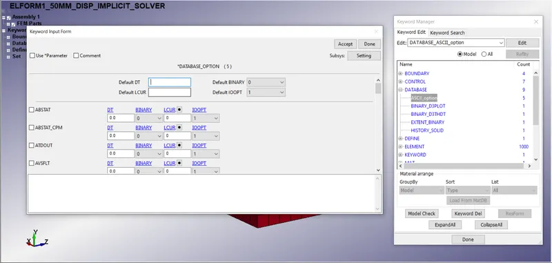
• *DATABASE_ASCII_option:-

The time step value of 0.005ms is given for GLSAT, MATSUM, ELOUT.

9) Checking Model:-

Go to Model Checking > Keyword Check.

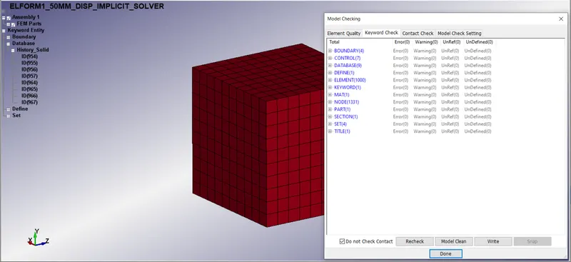
As we can see here that everything looks fine and there is no error. We can save this final .k file to run in LS-Run.

10) Running the .k file:-

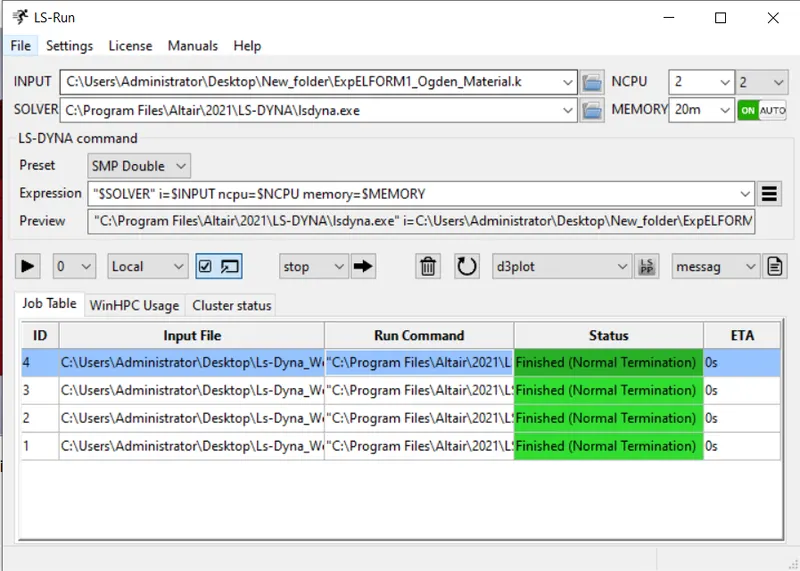
Run the saved keyword file of Element formulation 1 using LS-Run. If it is a Normal termination, post processing is carried out. If it is an error termination, recheck the model.

If it is a normal termination, then change the element formulations to 2, -1 and -2 individually in any of the text editor and run the model using LS-Run.

RESULT:-

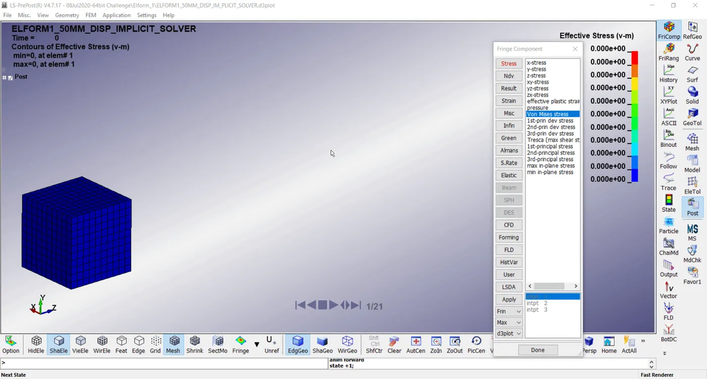
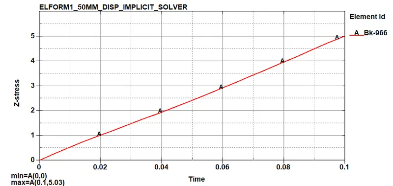
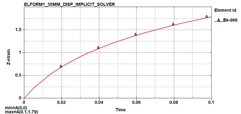
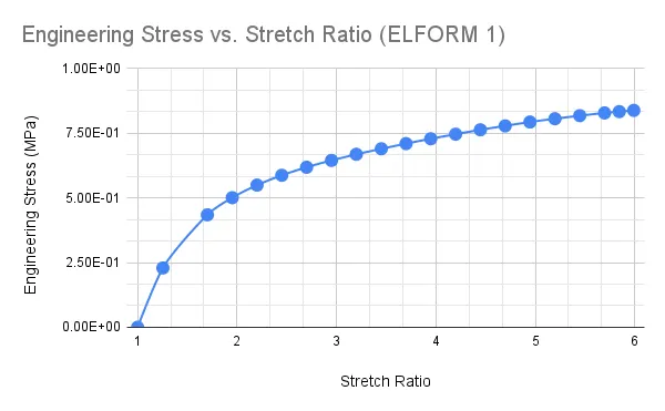
1) ELFORM 1

Max. Stress - 5.027 (gm/mm.ms^2)

Max. Strain - 1.7903

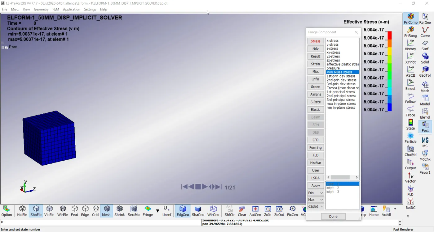
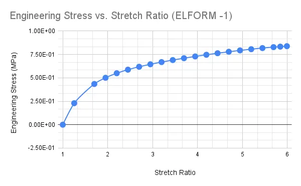
2) ELFORM -1

Max. Stress - 5.0253 (gm/mm.ms^2)

Max. Strain - 1.7905

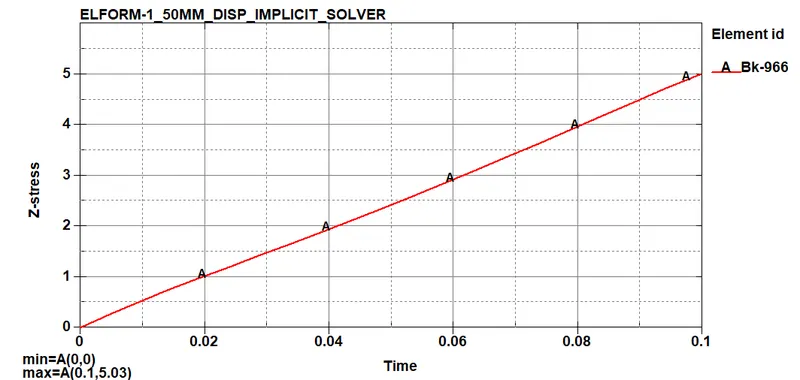
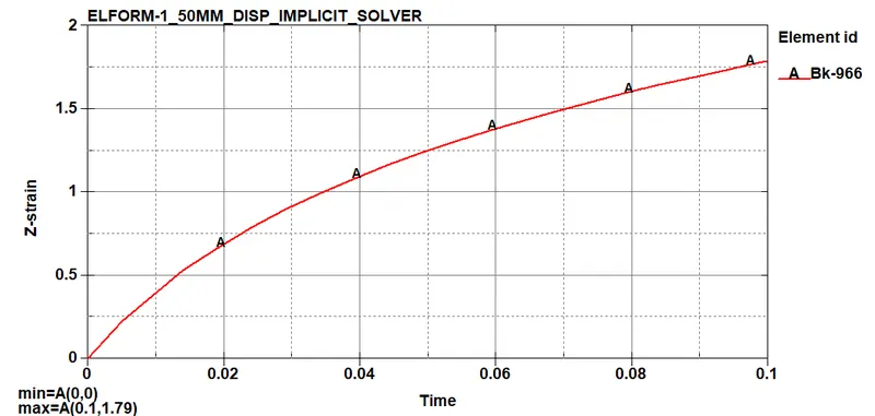
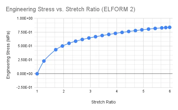
3) ELFORM 2

Max. Stress - 5.027 (gm/mm.ms^2)

Max. Strain - 1.7903

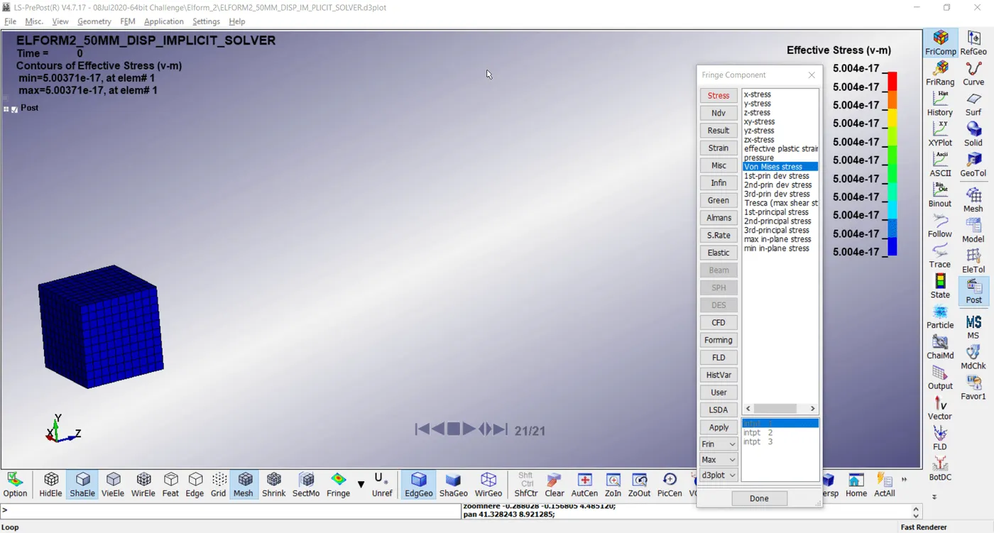
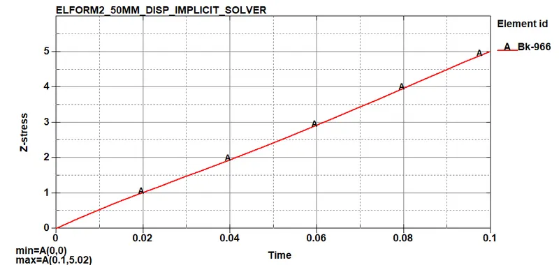
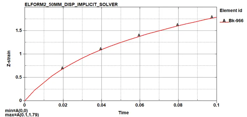
4) ELFORM -2

Max. Stress - 5.0235 (gm/mm.ms^2)

Max. Strain - 1.7903

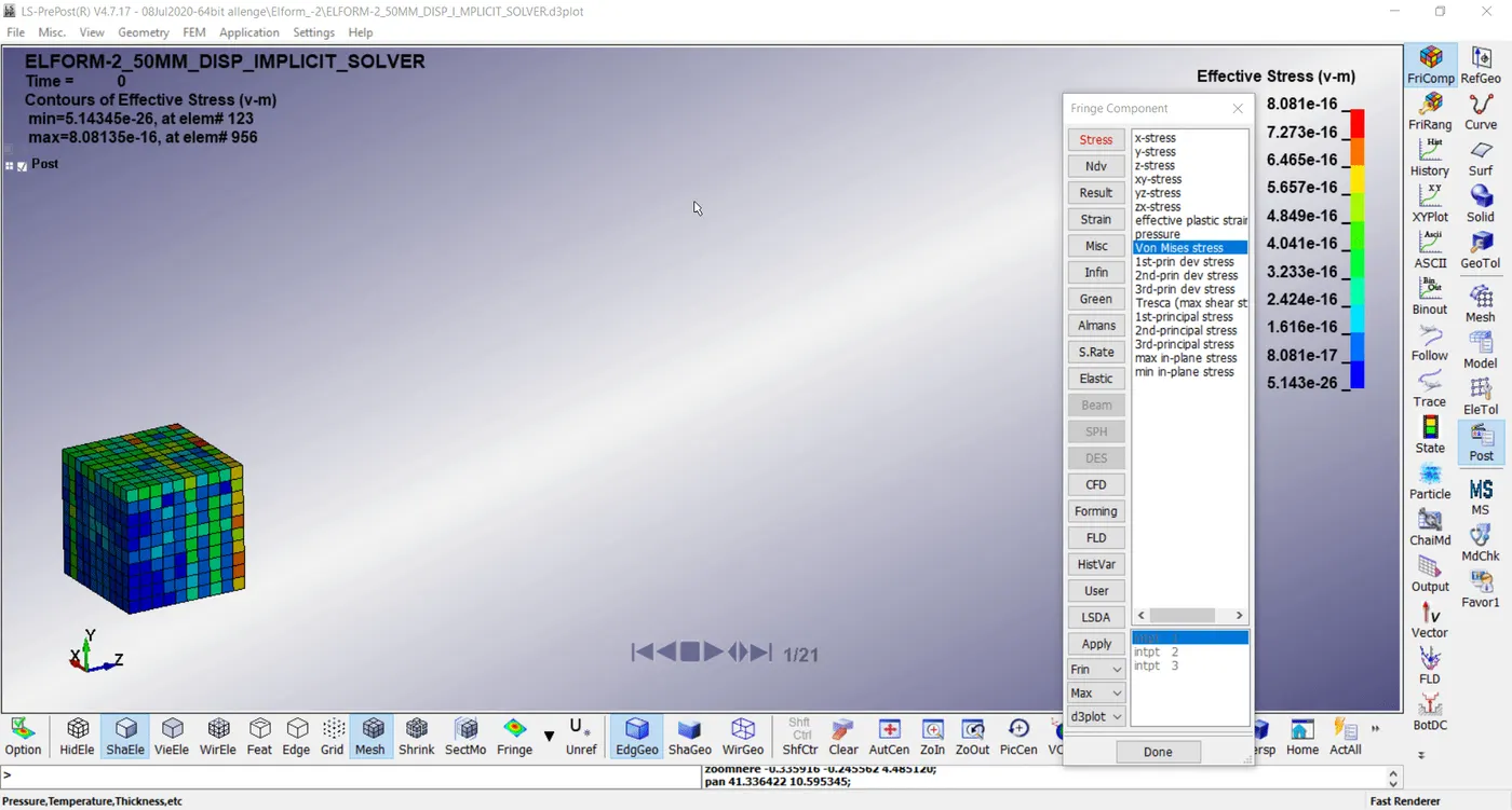
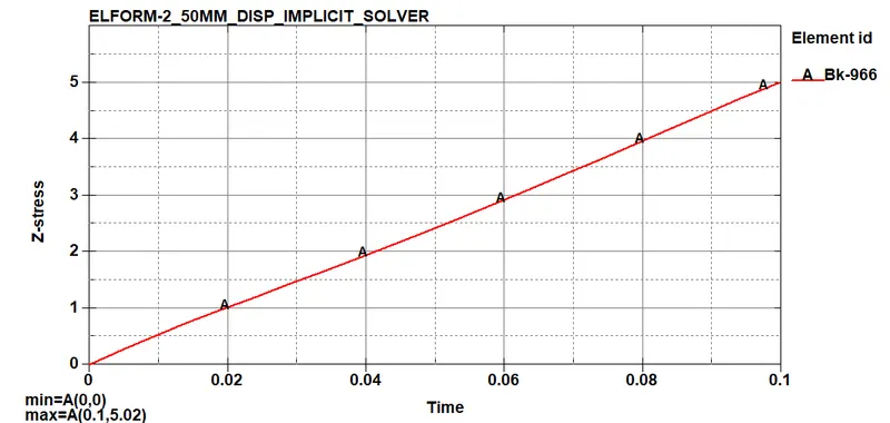
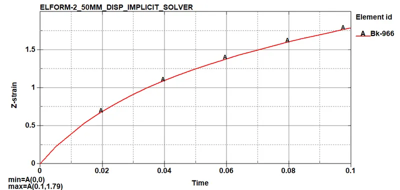
In LS-DYNA the output of stress and strains from Post Fringe Comp Stress/Strain is given as true stress and strains. To find the engineering stress/strain and stretch ratio following relations are used,

We know that,

1) True stress = Engineering Stress*(1 + Engineering Strain)

Engineering Stress = True Stress/(1 + Engineering Strain)

2) Engineering Strain = e^(True Strain) - 1

3) Stretch Ratio = 1 + Engineering Strain

ELFORM 1

ELFORM -1

ELFORM 2

ELFORM -2

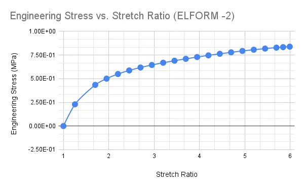
From the graphs plotted for Engg. Stress vs Stretch Ratio for different cases, the Engg. stress value corresponding to a stretch ratio of 5 is 0.8 MPa approximately. The output from different cases of elforms gives approximately same results since the model and loading conditions are simple. The actual plot for nominal stress vs stretch ratio for ogden material is shown in fig. mentioned in the objective. In the actual plot the value of nominal stress for a stretch value of 5 is approximately 1.8 MPa but from the simulation result the value of stress is 0.8 MPa. It is observed that a variation of 1 MPa is caused in the simulation for uniaxial tension test for ogden material because of non-linearity of the material and relatable boundary condition applied for the model.

CONCLUSION:-

• A FE model of solid block was created with ogden material to simulate uniaxial tension test for different cases of ELFORM (1, -1, 2, -2).
• The Engineering stress/strain and stretch ratio was calculated to plot a graph of Engg. stress vs stretch ratio up to stretch ratio 5.
• The Engineering stress value for a stretch value 5 from the simulation for different ELFORM was approximately equal to 0.8 MPa, but from the actual graph it was equal to 1.8 MPa with a difference of 1 MPa.
• The uniaxial tension test was solved using Implicit Solver since the analysis is similar to a quasi-static analysis on a hyperelastic non-linear material with slow steady loading conditions.