Week-6 Calculate the Stretch Ratio by comparing the ELFORM (-2,-1,1,2) with Ogden_Material Model.

Aim : To simulate tensile behaviour for the model (10x10x10 mm³) solid elements and compare among different element formulation of a hyperelastic material Ogden.

Explaination:

Stretch ratio is defined as the ratio of final length to the initial length of a component. Since the initial length is 10 mm and the simulation is to be carried out upto a stretch ratio of 5. The final length can be calculated using the formula to arrive at 50 mm.

The loading can be ramped from 0 mm to 50 mm displacement in 0 to 1 step. Since, the loading in tensile test is steady i.e equal displacement in equal interval of time.

PRE-PROCESSING :

(1) Modelling/ Discretization :

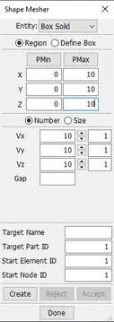
A 10mmx10mmx10mm solid cube is created using shape mesher from Elements and mesh tab.

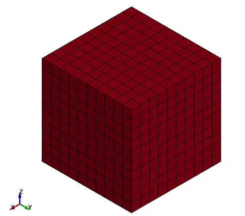
Meshed solid cube

(2) Section properties :

The section properties of the cube is chosen as follows.

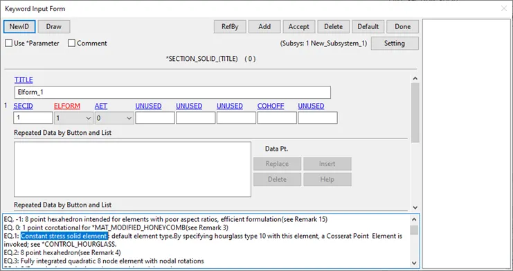
The element formulation elform=1 (default element type), i.e Constant stress solid element is used to run the initial simulation. In the subsequent simulation, this value is changed as -1, 2 and -2 by editing the keyword file.

(3) Material properties :

The material properties are saved in a keyword, which can be imported to the current keyword file by using include keyword.

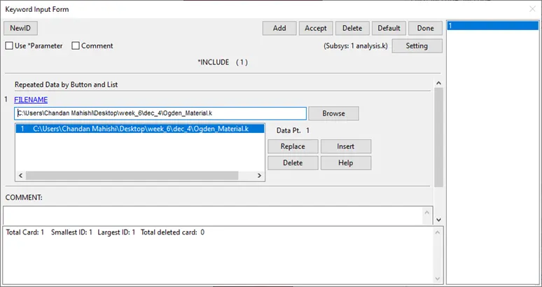
The material keyword is created using the material keyword file. This is Hyperelastic non-linear material called Ogden with following properties.

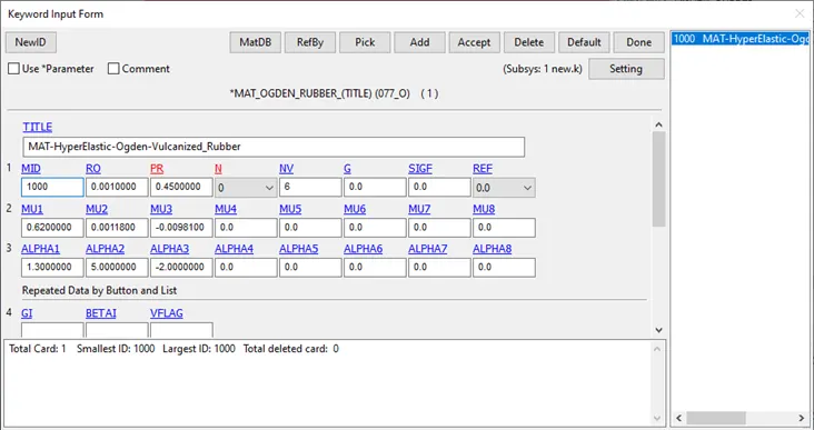
Ogden material

(3) Boundary conditions/Constraints/Loads:

Boundary conditions:

To simulate a uniaxial tensile test, one side of the specimen is held fixed in the collet and load is applied at the other end.

Likewise, one end is constrained to move along one direction and constrained in rest of directions i.e locked in 2 translational directions and 3 rotational direction.

This can be done by either creating an entity nodesetid followed by then a SPC_set keyword or directly creating SPC_set keyword and selecting nodes.

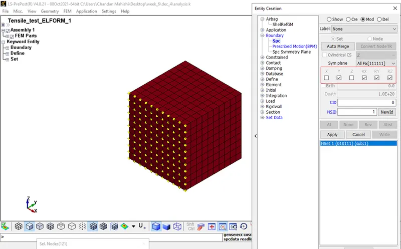
Since the loading is to be applied along positive y direction, the end nodes on the other side of cube in x-z direction are constrained in y and rotational dof.

Since this is a solid element, to simulate the real time boundary condition and to prevent any numerical instability, the mid nodes along transverse direction are also constrained along with the rotational degrees of freedom.

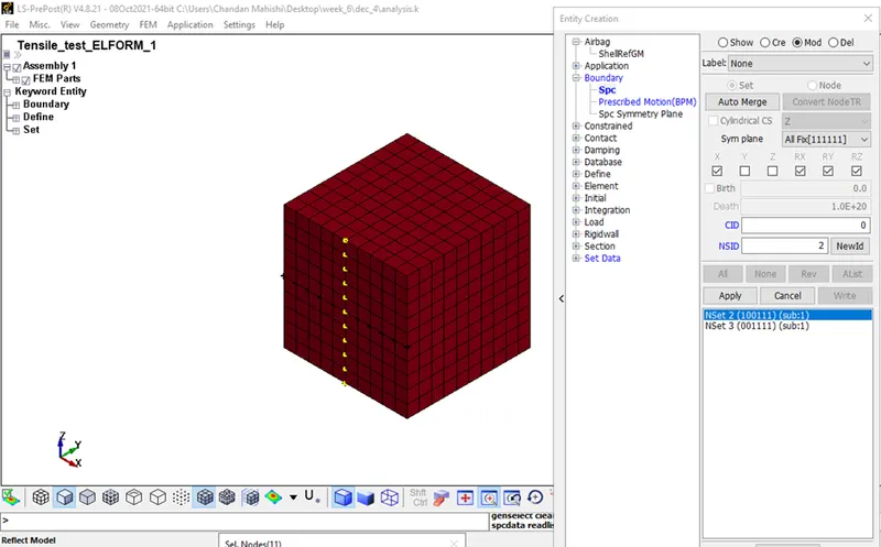
Constrained in x-direction and rotational degree of freedom

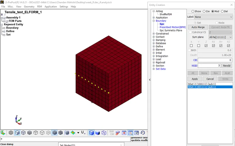
Constrained in z-direction and rotational degrees of freedom

Load:

To simulate the tensile test, a curve is defined as calculated from stretch ratio. The curve is defined from the Define keyword. The load is ramped from 0 to 50 mm in 1 step, an additional constant load after 1 is added to overcome numerical instability if any.

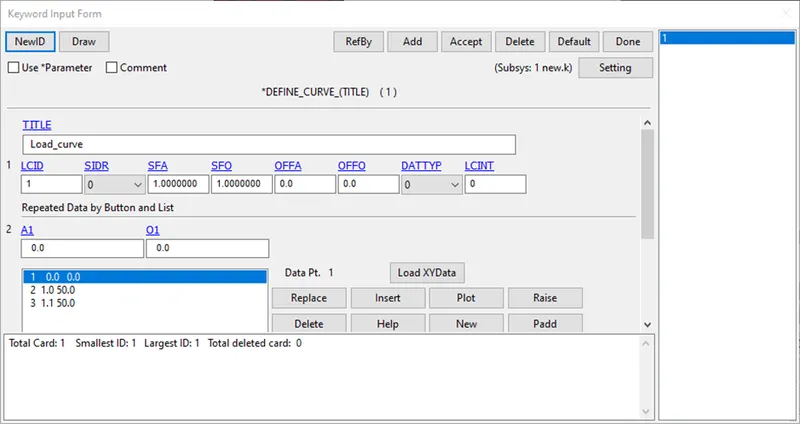
The loading is the form of displacement is applied to the other end of cube from Prescribed_motion_set keyword from Boundary keyword.

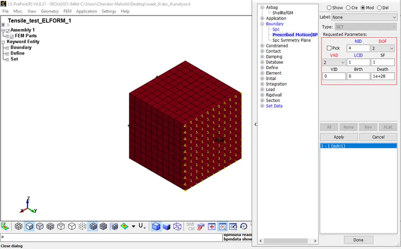
Since the loading is in form of displacement, VAD is selected as 2 and DOF is selected as 2(along y). The LCID represents load curve id which was defined in the previous step.

(5) Control :

Implicit general:

As tensile test is a steady state test (equal load/displacement in equal intervals of time), we run an implicit analysis. On the other hand, to run an explicit analysis time step should be very small. if the time increment becomes too large, then method becomes unstable and the error on the solution increases exponentially.

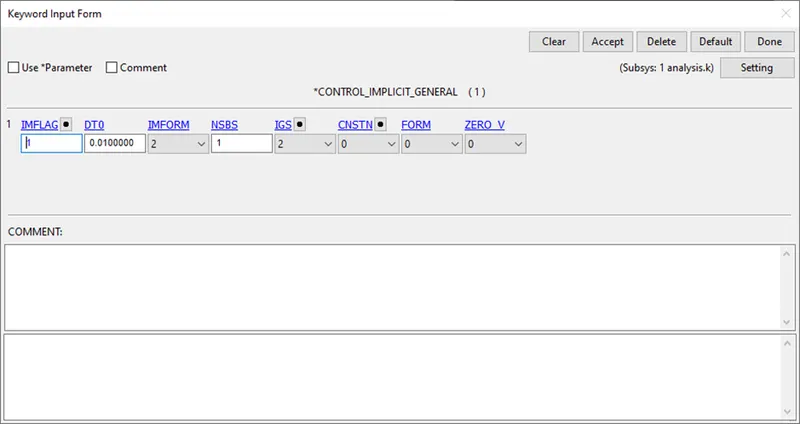
To activate implicit analysis Control_Implicit_General keyword is to be added. IMFLAG = 1 activates the implicit analysis. DT0 is initial time step that is to be defined.

Solving implicit analysis is an incremental iterative method with an initial guess. The solver looks for equilibrium based on displacement and energy i.e iterations in every increment of load.

The intial guess/ timestep is DT0 that we define. As a thumb rule, it should be endtime/100 (i.e 0.01).

This is to be selected so that convergence is achieved, which is a trade-off between many steps, few iterations (expensive) and few steps, many iterations (unreliable).

Implicit auto:

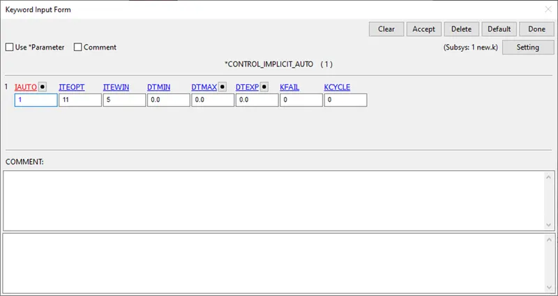
Implicit auto used to fine tune the solver. IAUTO is used to automatically adjust time step size in order to lessen the number of load increments. ITEOPT and ITEWIN are used to either increase or decrease the load increments. These have to be cautiously selected so as to run the solution in unreliable or expensive condition.

ITEOPT is used to limit the number of iterations required for a particular load increment or optimum iterations required. Increase or decrease in timestep depends on equilibrium achieved between ITEOPT-ITEWIN and ITEOPT+ITEWIN respectively.

DTMIN and DTMAX are bounding parameters which allow the minimum and maximum step based on the intial timestep (DT0) defined. Both of them can be left default but a good way to control would be DTMIN to be DT0/100 and DTMAX to be DT*10.

Implicit solution:

NSOLVER is used to select the solution method for implicit analysis. Since the material is non linear, Nonlinear with BFGS updates + optional arclength solver (NSOLVER =12) can be used with rest of parameters left default.

DCTOL and ECTOL are tolerance within the residuals can lie. These two can be varied depending on accuracy required with trade-off between unreliable and expensive way.

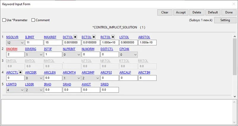
Implicit solver:

Implicit solver is used to invert the stiffness matrix in each iteration to check for residuals. The default Parallel multi-frontal sparse solver is used with LCPACK library.

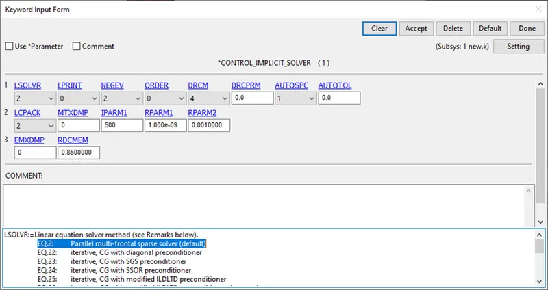
Termination:

Control termination keyword is used to denote the end time as 1.

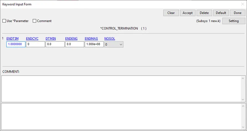
(6) Database :

Binary D3Plot is written for every 0.1 unit interval of time. Extent binary is used to derive strain tensor data by denoting STRFLAG as 1.

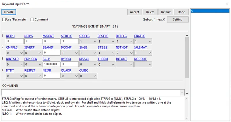
(7) Part :

In this section, the different parts/components in the file are connected to their respective material ID and section ID.

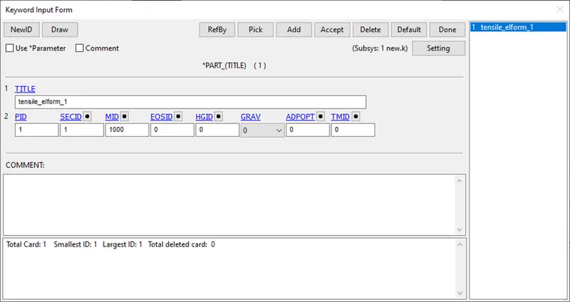
Once all the above is done, Model check is done to ensure all the parts are connected to their respective material, section are all well defined. A dialog box containing the cards - the errors, warnings, unreferenced, undefined are displayed. Approppriate action should be taken to overcome errors and warnings can be minimised.

SOLVING :

The above created input file is saved as keyword file (.k extension). This keyword file is solved using LS DYNA manager.

POST PROCESSING :

Various contour plots are plotted to check for sanity of the problem being solved. The animated file of the problem can be checked by running the d3plot file in the LS-PrePost.

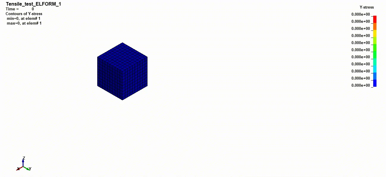
Analysis:

The simulation is carried out by changing elform by editing the keyword file. The simulation was run by tuning initial time step from 0.01, 0.05 and 0.08. The results presented here is with initial timestep of 0.01. The results were requested for a particular element and results were extracted by using ASCII plot and saved in the folder. The extracted results were imported in the excel file. Since, LS Dyna reports true stress and strain values, engineering stress and strains are extracted by using the following formula.

True Strain (MPa)
Time step	ELFORM_1	ELFORM_-1	ELFORM_2	ELFORM_-2
0	0	0	0	0
0.153874	0.546923	0.546913	0.546913	0.546913
0.253874	0.780883	0.78076	0.78076	0.78076
0.353874	0.96488	0.963757	0.964777	0.96478
0.453874	1.11504	1.115037	1.115027	1.115023
0.553874	1.24002	1.240147	1.240007	1.240107
0.653874	1.34595	1.345747	1.345924	1.34592
0.753874	1.43611	1.436247	1.435993	1.436227
0.853874	1.513787	1.514238	1.51384	1.513693
0.953874	1.581403	1.58116	1.581143	1.581437
1	1.609177	1.609383	1.609323	1.609253

True Stress
Time step	ELFORM_1	ELFORM_-1	ELFORM_2	ELFORM_-2
0	0	5E-17	5E-17	5.77E-16
0.153874	0.8035	0.80349	0.80349	0.80349
0.253874	1.2706	1.2702	1.2702	1.2702
0.353874	1.7313	1.7249	1.7309	1.7309
0.453874	2.2022	2.2021	2.2019	2.2019
0.553874	2.6906	2.6916	2.6904	2.691
0.653874	3.202	3.2005	3.2016	3.2015
0.753874	3.727	3.7274	3.7224	3.727
0.853874	4.2566	4.2625	4.2564	4.2556
0.953874	4.7892	4.7856	4.7851	4.7876
1	5.0222	5.0239	5.0232	5.0212

True strain, ɛ_t = ln(1+ ɛ_e)

Engineering strain, ɛ_e = e^ɛ_t -1

True stress, σ_t = σ_e(1+ ɛ_e)

Engineering stress, σ_e = σ_t/(1+ ɛ_e)

Stretch ratio is then calculated using the formula,

Stretch ratio = 1 + engineering strain

Engineering strain	Stretch ratio	Engineering stress (MPa)
ELFORM_1	ELFORM_1	ELFORM_1
0	1	0
0.727929	1.727929	0.465008
1.1834	2.1834	0.581936
1.624473	2.624473	0.659675
2.04969	3.04969	0.722106
2.455683	3.455683	0.778601
2.841835	3.841835	0.833456
3.20431	4.20431	0.886471
3.543905	4.543905	0.936771
3.861774	4.861774	0.985072
3.998696	4.998696	1.004702

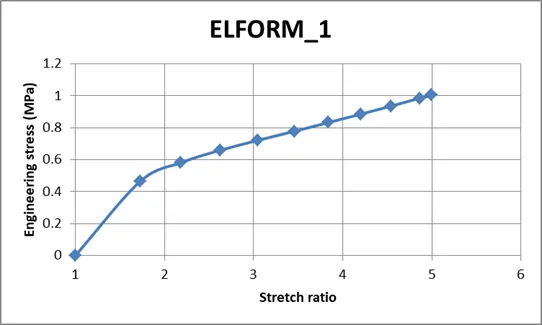
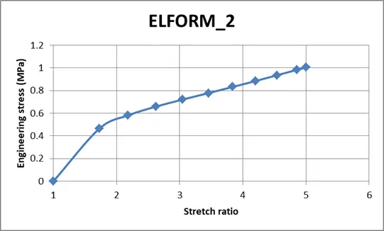
Accordingly, this is done for all the Element formulation and a graph of Engineering stress(Nominal) against stretch ratio is plotted.

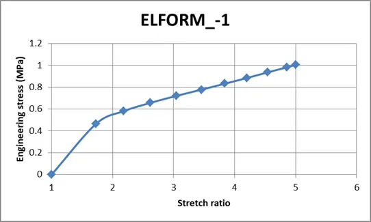
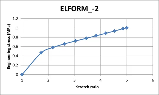
Results:

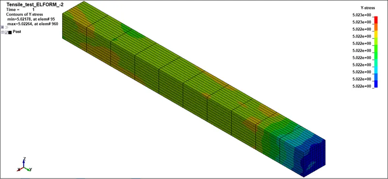
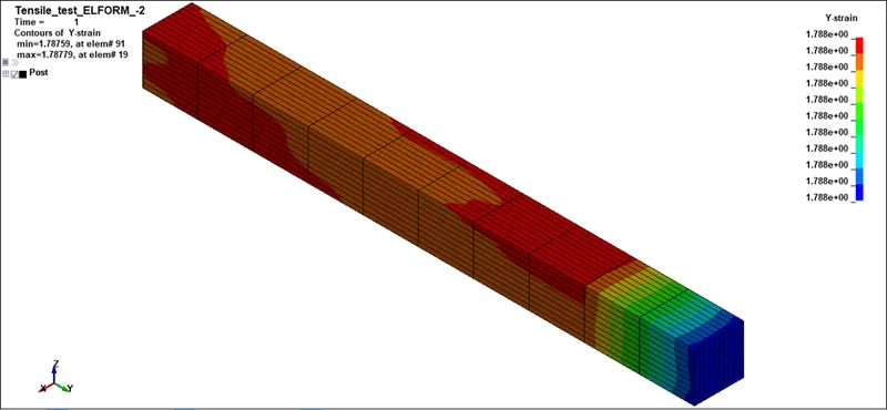
Elform 1 : Constant stress solid element.

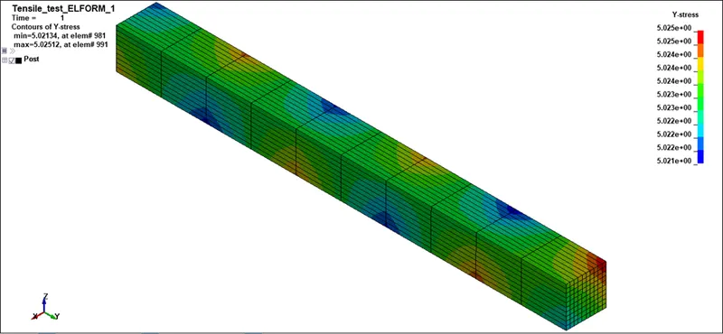
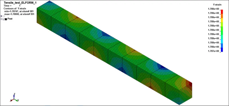
Elform 2: 8 point hexahedron

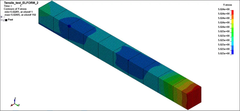
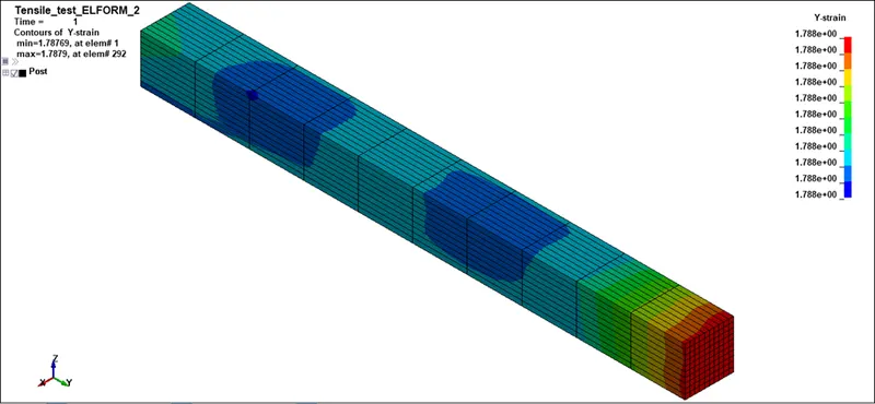
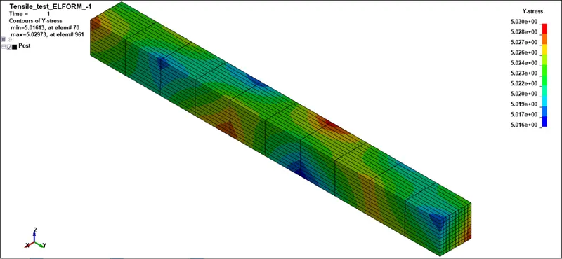
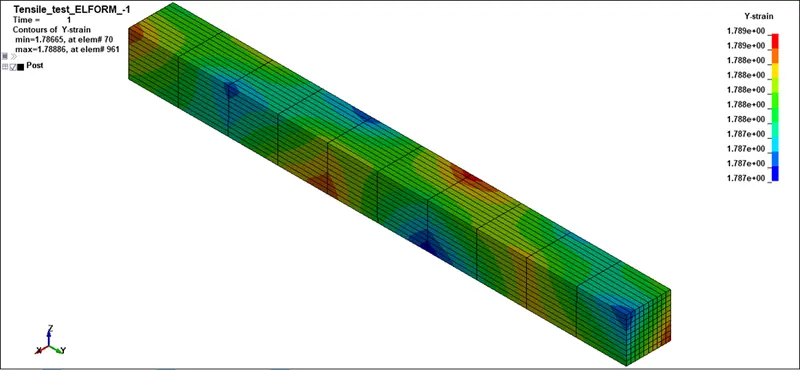
Elform -1: 8 point hexahedron intended for elements with poor aspect ratios

Elform -2: 8 point hexahedron intended for elements with poor aspect ratios

Conclusion:

Comparing the plot of Stress vs Stretch ratio for various element formulation, there is no significant difference in either the number of load steps required for convergence or variation in the results.

Elform 1 : Constant stress solid element.

It is efficient and accurate. Works well with severe deformation but needs hourglass stabilization.

Elform 2: 8 point hexahedron

It is slower than Elform 1, becomes stiff in case of poor aspect ratio, may result in shear locking and unstable in large deformation but doesn’t need hourglass stabilization.

Elform -1: 8 point hexahedron intended for elements with poor aspect ratios

It is identical with type 2, but accounted for poor aspect ratio in order to reduce shear locking.

Elform -2: 8 point hexahedron intended for elements with poor aspect ratios

It is identical with type 2, but accounted for poor aspect ratio in order to reduce shear locking but with higher computational cost than elform -1.

Though there is change in the way of calculation for different element formulation, the stress and strain values in the above plots are identical because of the simple model with elements having good aspect ratio that is there is no much variation in the values and taken for convergence are comparable.

Please follow the link to access the input, output and excel report : https://drive.google.com/drive/folders/1OnzLHChNmeZk4lJrcA21MvZU8amzBSeV?usp=sharing